Modeling the transport of radionuclides through the Culebra Dolomite Member of the Rustler Formation (hereafter referred to as the Culebra) is one component of the performance assessment (PA) performed for the U.S. Department of Energy (DOE) Waste Isolation Pilot Plant (WIPP) 2014 Compliance Recertification Application (CRA). Transport modeling in PA requires flow velocity results from the Culebra groundwater flow model. This Appendix describes the process used to develop and calibrate the input parameter fields for the Culebra flow model. Calibrated model parameters are referred to broadly as "T-fields" (transmissivity fields), although more parameters than just transmissivity (T) were calibrated as part of the CRA-2009 Performance Assessment Baseline Calculation (PABC) model (Clayton et al. 2010). This appendix describes the process followed for the CRA-2009 (PABC), which was a major change from the process followed for CRA-2004 PABC (Leigh et al. 2004), and involved a hydrology conceptual model peer review. The T-fields developed for CRA-2009 PABC were used unchanged in CRA-2014. Figures illustrating each calibrated T-field are given in Attachment A to this Appendix.
The work described in this Appendix was performed under two Sandia National Laboratories (SNL) analysis plans (APs): AP-114 (Beauheim 2008) and AP-144 (Kuhlman 2009). AP-114 (evaluation and recalibration of Culebra transmissivity fields) dealt with the development and calibration of the T-fields (including T, storativity (S), horizontal anisotropy (A), and vertical recharge (R)), in addition to development of T-field acceptance criteria. AP-144 (calculation of Culebra flow and transport) dealt with the modification of T-fields for the potential future effects of potash mining for use in the PA Culebra radionuclide transport calculations. The PA Culebra radionuclide transport calculations are not described in this Appendix, which focuses on the development and modification of the T-fields.
West of the WIPP, Culebra T is high where the Culebra overlies areas where the Salado Formation has been removed by dissolution (mostly in Nash Draw). East of the WIPP, Culebra T is low when the Culebra is bounded either above or below by halite in adjoining Rustler units. Further to the east, Culebra T is very low when the Culebra is bounded both above and below by halite in the Rustler. At the WIPP, between the high T in the west and low T in the east, Culebra T is observed to change significantly over short distances and is simulated in the WIPP Culebra flow model using a random mixture (i.e., stochastic patches) of high and low T zones, consistent with geologic and hydrologic observations. The geologic data discussed in Section TFIELD-2.0 are used to specify the boundaries of these Culebra conceptual model zones (Section TFIELD-3.0), which are then carried forward into the numerical implementation of the Culebra groundwater model (Section TFIELD-4.0).
The starting point in the T-field development process was to assemble and update information on geologic factors potentially affecting Culebra T (Section TFIELD-2.0). These factors include dissolution of the upper Salado Formation located below the Culebra, presence of gypsum cements, the thickness of overburden above the Culebra, and the spatial distribution of halite in the Rustler Formation both above and below the Culebra. Geologic information is available from hundreds of oil and gas wells and potash exploration holes in the vicinity of the WIPP site, while estimates of Culebra T are available from only 64 well locations. Details of the geologic data compilation are given in Powers (Powers 2002a, Powers 2002b and Powers 2003), updated in Powers (Powers 2007a and Powers 2007b), and summarized in Section TFIELD-2.0.
A two-part geologically based approach was used to generate base Culebra T-fields. In the first part (Section TFIELD-3.0), a conceptual model for geologic controls (i.e., soft data) on Culebra T was formalized and the hypothesized geologic controls were regressed against Culebra T estimates at monitoring wells to determine linear regression coefficients. The regression includes one continuously varying function, Culebra overburden thickness, and three indicator functions that assume values of 0 or 1 depending on the occurrence of open, interconnected fractures; Salado dissolution; and the presence or absence of halite in Rustler units bounding the Culebra.
In the second part (Section TFIELD-4.0), a method was developed for applying the linear regression model to predict Culebra T across the WIPP model area between the sparse observations at wells. The regression model was combined with the maps of geologic factors to create 1,000 stochastically varying base Culebra T-fields. Details about the development of the regression model and the creation of the base T-fields are given in Hart et al. (Hart et al. 2008). The conceptual model embodied in these 1,000 base Culebra T-fields was subject to peer review before model calibration proceeded (Section TFIELD-3.7). The peer review panel concluded the justification and scientific rigor of the methodology for preparing base T-fields were adequate (Burgess et al. 2008). A sample of 200 out of the 1,000 created base T-fields were calibrated following the process outlined in Section TFIELD-5.0, with the 100 best calibrated T-fields eventually chosen for use in PA radionuclide transport calculations.
Section TFIELD-5.0 presents details on the modeling approach used to calibrate the T-fields to both steady-state heads across the model domain and transient drawdown measurements from multi-well pumping tests. Heads measured in 42 Culebra observation wells around May 2007 were used to represent steady-state conditions in the Culebra, and drawdown responses in 67 total observation wells (62 unique locations) across nine pumping tests were used to provide transient calibration data. See Appendix HYDRO-2014 for more information on the Culebra monitoring well network and recent trends observed in Culebra water levels. Details on the steady-state heads are described in Johnson (Johnson 2009a and Johnson 2009b), and the transient drawdown data are summarized in Hart et al. (Hart et al. 2009). Assumptions made in modeling, the definition of an initial head distribution, assignment of boundary conditions, discretization of the spatial and temporal domain, weighting of the observations, and the use of PEST (Doherty 2000) with MODFLOW-2000 to calibrate the T-fields using a pilot-point method are described in detail in Hart et al. (Hart et al. 2009) and summarized in Section TFIELD-5.0.
Section TFIELD-5.3.4 addresses the development and application of acceptance criteria to select the 100 best T-fields from the 200 calibrated T-fields. Acceptance was based on a combination of objective fit to both the steady-state and transient pumping test calibration data. Section TFIELD-5.4 provides summary statistics and other information for the 100 T-fields that were judged to be acceptably calibrated. Attachment A presents T, S, diffusivity (D), and model-predicted flow speed for each of the chosen 100 realizations.
The data used in the construction (Sections TFIELD-3.0 and TFIELD-4.0) and calibration (Section TFIELD-5.0) of the T-fields were divided into three groups:
- soft data only used in base T-field generation,
- hard data used in both T-field generation and calibration, and
- hard data only used in calibration.
This first group included geologic data (i.e., Salado dissolution, presence of gypsum cements in the Culebra, Culebra overburden thickness, and the locations of Rustler halite margins) and hydrologic data (i.e., pairs of pumping and observation wells interpreted to have high diffusivity from multi-well pumping tests). The soft data were included in T-field generation because they were used to define boundaries also used in the calibration phase. The second group only included estimated T from single-well pumping tests, which were used directly in indicator kriging, indirectly in the overburden regression analysis, and directly as fixed pilot points in the calibration phase. The third group only included head and drawdown observations used as calibration targets. Some of these third group data were used in other analyses to estimate diffusivity values used as soft data (first group), but the drawdown data from multi-well pumping tests only appeared directly in the calibration phase.
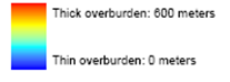
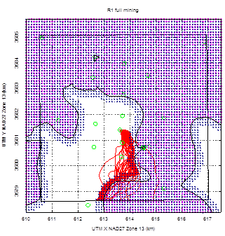
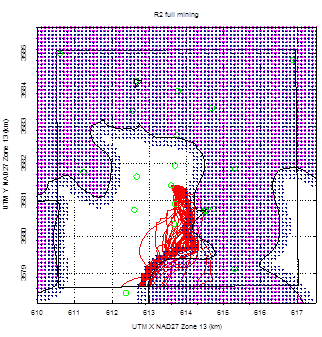
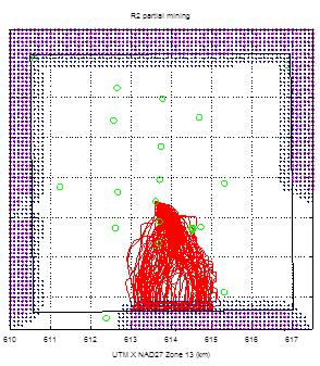
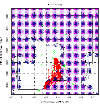
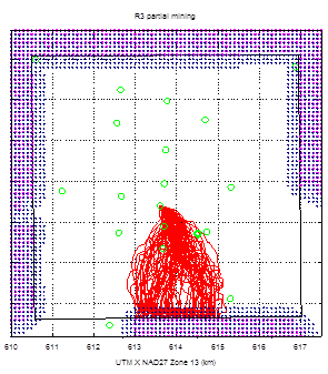
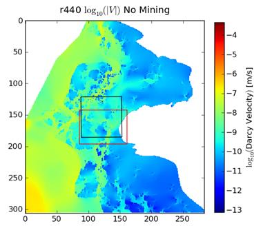
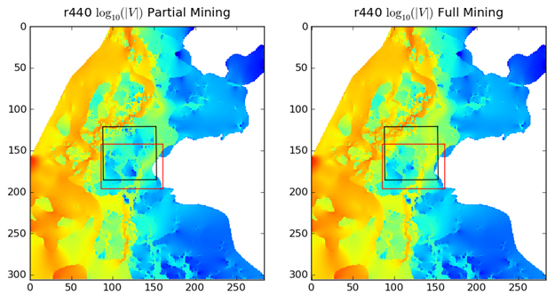
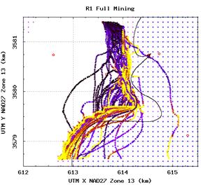
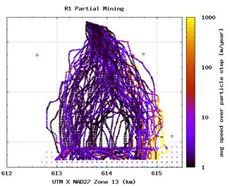
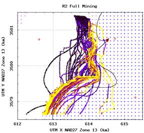
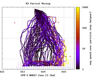
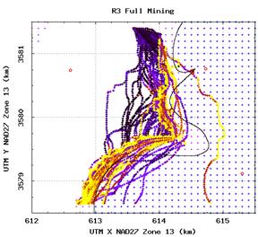
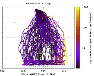
Section TFIELD-6.0 discusses modifications of the T-fields performed to account for the effects of potash mining both within and outside the WIPP land withdrawal boundary. Potentially mining-affected areas were delineated, random transmissivity multipliers were applied to the transmissivity field in those areas, and particle tracks and travel times were computed (Kuhlman 2010). The flow fields produced by these mining-affected T-fields were input to the radionuclide transport model SECOTP2D used to compute both CRA-2009 PABC and CRA-2014 long-term PA releases (Appendix PA-2014). Section TFIELD-7.0 provides an executive summary of the development and modification of the Culebra T-fields.
The work outlined in Section TFIELD-2.0 was performed as Task 1 under AP-114, Analysis Plan for Evaluation and Recalibration of Culebra Transmissivity Fields (Beauheim 2008). There were no changes to the model between CRA-2009 PABC and CRA-2014. Geologic data were updated to improve definition of geologic boundaries used to define zones as part of the process of creating new T-fields. Geologic boundaries were refined for CRA-2009 PABC using data from field investigations and newly obtained oil and gas well log data (Section TFIELD-2.2). The Salado dissolution margin bounds the high-T Culebra zone to the west in Nash Draw, and was only modified slightly for CRA-2009 PABC. The Rustler halite margins bound the very low-T Culebra zone to the east, and were modified significantly for CRA-2009 PABC. The confinement of the Culebra in the southeastern portion of Nash Draw was also investigated in AP-114 Task 1, to constrain the Culebra flow model inputs (Section TFIELD-2.3). Previous to CRA-2009 PABC, the Culebra groundwater flow model was only steady-state and did not include input parameters related to confinement or recharge. A model was developed regarding distribution of gypsum cements in the Culebra from available core data (Section TFIELD-2.3.3).
The Culebra Member of the Rustler Formation is considered as a potential long-term release pathway in WIPP PA because it is the most permeable laterally continuous geologic unit above the WIPP repository level (see Figure TFIELD 2-1 for general stratigraphy). Potential future human intrusion into the repository might connect the repository with the Culebra, which would then transport radionuclides to the accessible environment under natural flow conditions. The accessible environment is defined to be where the WIPP Land Withdrawal Boundary (LWB) intersects the Culebra in the subsurface.
The ability of the Culebra to advect groundwater and radionuclides to the accessible environment is affected by both depositional and post-depositional effects. The Culebra is believed to have been deposited quite uniformly over a wide area (the vertical thickness of the Culebra is quite uniform over lateral distances of many miles (e.g., Holt and Powers 1988)), but depositional effects include the presence of mudstone or halite layers in the Rustler Formation immediately above and below the Culebra. Post-depositional processes include dissolution of halite from the underlying Salado Formation and precipitation of vug- and pore-filling evaporates within the Culebra (see Figure TFIELD 2-2).
Understanding of the spatial distribution and thickness of halite in the Rustler Formation was improved for CRA-2009 PABC (compared to CRA-2009 (U.S. DOE 2009)) due to data obtained from analysis of geophysical logs from oil and gas wells. The lateral extent of Salado dissolution was modified slightly for CRA-2009 PABC, but remained largely similar to CRA-2009, with minor adjustments due to additional information for a few new WIPP wells (Powers 2007a and Powers 2007b).
Groundwater flow in the Culebra is generally from north to south at the WIPP site. Water levels in Culebra wells in Nash Draw (several miles to the west of the WIPP site) respond more rapidly to precipitation and behave differently than Culebra wells in the immediate vicinity of the WIPP site (Appendix HYDRO-2014, Section 7.1
). Based on the north-south gradient currently observed at the WIPP, particle-tracking predictions from the WIPP waste panels through the Culebra result in flow towards the southern edge of the WIPP LWB.
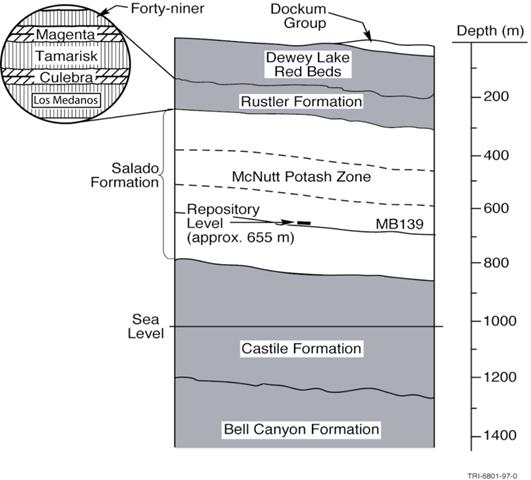
Figure TFIELD 2-1. Generalized Stratigraphy Near the WIPP
The locations of the Rustler halite margins (Section TFIELD-2.2.1) and the Salado dissolution margin (Section TFIELD-2.2.2) both affect the conceptual model of Culebra T (see Figure TFIELD 2-1 for general relationships between the Rustler, the Salado and the WIPP repository). These were updated as part of the CRA-2009 PABC geologic study.
The presence of halite in the non-dolomite members of the Rustler Formation correlates strongly with estimates of Culebra T. Halite and anhydrite are found as pore-filling cements in the Culebra (reducing open fractures) when halite exists in layers above the Culebra, below the Culebra, or both (Figure TFIELD 2-2). When halite is found either above (H3) or below (H2) the Culebra, observed Culebra T is low. When halite exists both above and below the Culebra, observed Culebra T is extremely low.
North, south and west of the WIPP site, Cenozoic dissolution has affected the upper Salado Formation. Where this dissolution has occurred, the rocks overlying the Salado, including the Culebra, are strained (leading to larger apertures in existing fractures), fractured, collapsed, or brecciated (e.g., Beauheim and Holt 1990). All WIPP Culebra wells within the Salado dissolution zone have been interpreted to have high T. It is hypothesized that all regions affected by Salado dissolution have well-interconnected fractures and therefore high T.
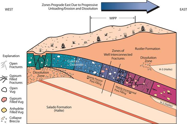
Figure TFIELD 2-2. WIPP Culebra Dolomite Conceptual Model. Culebra T decreases to the east (increasing overburden and halite) and increases to the west (fracturing due to underlying Salado dissolution). Halite appears both above (H-3) and below (H-2) the Culebra in the east. Primary groundwater flow direction through the Culebra is south.
The Rustler Formation stratigraphic column given in Figure TFIELD 2-3 shows two types of geologic variability. Vertical stratigraphy places older formations below younger formations at the same location in space (e.g., the Los Medaños Member is older than the Culebra Member), while facies change place two units of similar age at different spatial locations, due to changes in depositional environments (e.g., Mudstone 4 (M4) and Halite 4 (H4) of the Forty-niner Member are of the same age, but occur in different locations).
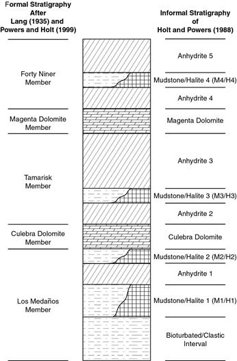
Figure TFIELD 2-3. Rustler Formation Stratigraphic Nomenclature
Powers (Powers 2002a and Powers 2002b) provided geologic data across the CRA-2004 PABC Culebra modeling domain that included maps of halite margins within the Rustler Formation. Those margins were largely based on work in Powers and Holt (Powers and Holt 1995), modified by some data collected from potash drillholes, especially in the northern area of the Culebra modeling domain. The observed distribution and thickness of halite in the Rustler is interpreted to be the result of sedimentary structures and facies relationships controlled by deposition, rather than the result of dissolution alone (Holt and Powers 1988; Powers and Holt 1999; Powers and Holt 2000). Before Holt and Powers (Holt and Powers 1988), many researchers incorrectly believed a uniform thickness of Rustler halite was deposited and later removed by dissolution in the areas near Nash Draw, leaving the observed mudstone layers as dissolution residue. Definitive data collected during WIPP air-intake shaft geologic mapping provided the basis for the current facies-based conceptual model used at the WIPP (Holt and Powers 1988). Some minor zones adjacent to the depositional margins have been interpreted as having undergone some post-depositional dissolution of halite, specifically the halite in the Tamarisk Member, but the extent of this Rustler halite dissolution is relatively minor (Beauheim and Holt 1990).
Significant changes to the locations of the M3/H3 and M2/H2 margins have been made for CRA-2009 in some areas since CRA-2004 (U.S. DOE 2004) as part of Task 1A of AP-114. The Rustler halite margins used since CRA-2009 PABC are shown over a wide area in Figure TFIELD 2-4 through Figure TFIELD 2-7, as defined in Powers (Powers 2007a and Powers 2007b). Changes in the location of the halite margins were based mostly on newly obtained geophysical log data obtained from oil and gas exploration (both new and old wells), and a few hydrologic wells drilled by the WIPP program since 2003 (Powers 2007a).
Wells H-17 and H-12 (see Figure TFIELD 2-8), located where halite occurs in the Tamarisk Member (H3 interval; Figure TFIELD 2-6) but not in the Los Medaños Member (M2 interval; Figure TFIELD 2-5) of the Rustler Formation show low transmissivity. We assume high-transmissivity zones do not occur in the Culebra where H2 or H3 also occur. Margins near the WIPP remain nearly unchanged, and all modifications to the margins do not change the basic interpretation that the margins are the result of deposition and local syndepositional dissolution of halite, not regional halite dissolution from the Rustler (Holt and Powers 1988; Powers and Holt 2000; Powers et al. 2006). Core evidence from well SNL-8 shows limited brecciation of anhydrite 3 in the Tamarisk (Figure TFIELD 2-3) that is interpreted as an extension of a narrow margin along the H-3 margin where a limited amount of halite was dissolved after deposition (Powers 2009).
After refining the Rustler halite margin locations, all mudstone/halite margins now show similar gross trends (compare Figure TFIELD 2-4 through Figure TFIELD 2-7 and Figure TFIELD 2-8). Southeast of the WIPP, the margins are elongate roughly northwest to southeast. The gross trends of these margins are similar to the trend in the elevation of the top of Culebra (Figure TFIELD 2-9). As previously described (e.g., Holt and Powers 1988); Powers et al. (Powers et al. 2003), this northwest-to-southeast trending anticlinal feature is called the Divide anticline. Mudstone dominates along this trend in three of the mudstone-halite units of the Rustler (i.e., all except M1/H1).
|
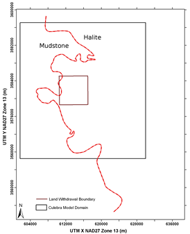
Figure TFIELD 2-4. M-1/H-1 Halite Margin In the Lower Los Medaños Member
|
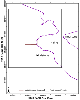
Figure TFIELD 2-5. M-2/H-2 Halite Margin In the Upper Los Medaños Member
|
|
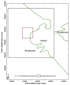
Figure TFIELD 2-6. M-3/H-3 Halite Margin In the Tamarisk Member
|
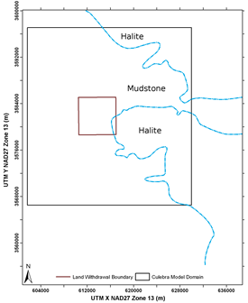
Figure TFIELD 2-7. M-4/H-4 Halite Margin In the Forty-niner Member
|
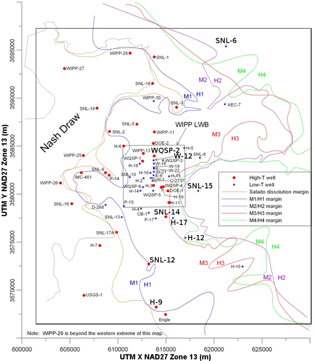
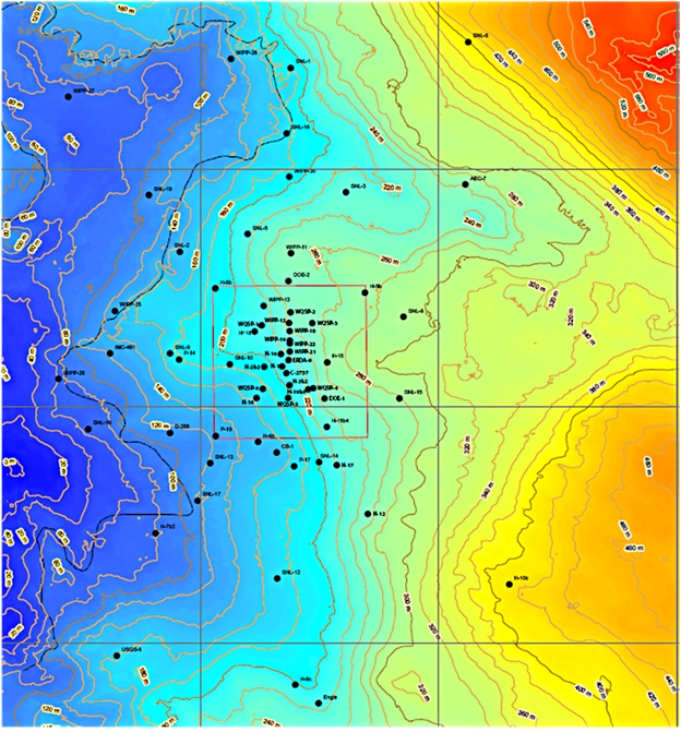
Figure TFIELD 2-8. Salado Dissolution Margin and Rustler Mudstone/Halite (M/H) Margins. WIPP Culebra wells with high or low transmissivity (T) are indicated. WIPP Culebra model extents indicated with large black rectangle. Wells mentioned in text are labeled using larger font.
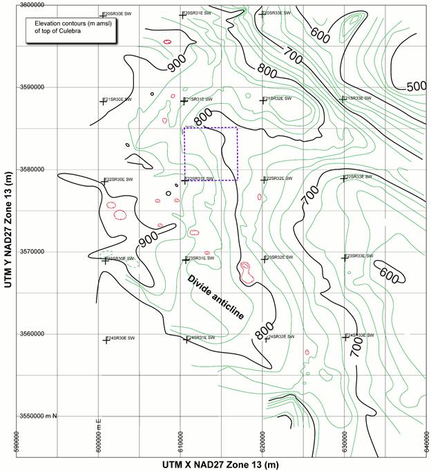
Figure TFIELD 2-9. Top Elevation (m Above Mean Sea Level (AMSL)) of the Culebra. WIPP LWB indicated with blue dashed line. Township (T) and Range (R) corners indicated with crosses.
A margin marking the lateral extent of significant dissolution of upper Salado Formation halite for CRA-2004 PABC was inferred from significant local changes in thickness of the interval between the Culebra Dolomite and the Vaca Triste Sandstone Member of the Salado (Powers 2002a and Powers 2002b). For CRA-2009 PABC, the margin was modified to reflect information indicating embayments of the dissolution margin. Additional data were added south of the WIPP, with log cross sections, to delineate the margin more accurately (Powers 2003). Some of these data are reflected in the simplified maps included in Powers et al. (Powers et al. 2003) and Holt et al. (Holt et al. 2005).
The Salado dissolution margin was updated for CRA-2009 (see Appendix G from the Analysis Report for Task 5 of AP-114 (Hart et al. 2008)) based on reinterpretation of geophysical borehole logs from oil and gas wells in the vicinity of H-9, which were not available for CRA-2004 PABC. This analysis placed H-9 east of the dissolution line, where previously it was considered to be within the area affected by Salado dissolution. The Salado dissolution margin is shown with the Rustler halite margins in Figure TFIELD 2-8, reflecting the change near H-9.
Field and map studies were performed to identify potential recharge locations south and west of the WIPP in the southeastern arm of Nash Draw (Powers 2006). This work also identified Culebra unconfined regions in the same geographic area. The boundaries to the west and south correspond to the model domain; the northern and eastern boundaries included the southeastern arm of Nash Draw and an area beyond the apparent eastern extent of the draw.
Five elements were identified as contributing to understanding recharge, which might be useful for modeling the possible effects of recharge to the Culebra in the study area:
1. extent of and relationship between surface drainage basins,
2. areas with differing Culebra confinement,
3. location and character of drainage channels within drainage basins,
4. location of specific recharge points (e.g., sinkholes), and
5. soil characteristics and rainfall infiltration across the study area.
Of these, the estimate of Culebra confinement is the most interpretive element. Drainage basins, channels and specific points of recharge are identified using surface topography features identifiable from maps, aerial photos, or field reconnaissance. Existing maps of soils, combined with surface reconnaissance and aerial photographs, permitted relatively direct assignment of soil properties controlling runoff. The degree of confinement of the Culebra in the study area, however, was not directly determinable from the surface data. As a result, a variety of surface features and well data were combined to estimate areas where the Culebra is less confined compared to conditions at the WIPP site, where there are more well-test and drillhole data.
Drainage basin size and characteristics are important elements to determine how rainfall, infiltration, and runoff may contribute to recharge of near-surface Rustler hydrologic units in Nash Draw. Topographic maps, aerial photographs, and some field checking were used to define separate surface drainage basins.
The drainage basins are mainly separated by topographic divides and local lows or concentration points that can be distinguished on 7.5-minute quadrangle topographic maps supplemented by study of aerial photographs. Because Nash Draw is an area of significant evaporite karst (e.g., Powers and Owsley (Powers and Owsley 2003)), collapse features, caves, or sinkholes may capture local drainage in smaller basins or subbasins wholly enclosed by another basin (Figure TFIELD 2-10). An example is drainage basin 7, which is wholly enclosed in drainage basin 6 (Figure TFIELD 2-10). These quite localized closed drainage basins in Nash Draw represent potential recharge locations for the Rustler Formation. Mapping the basins is the first step in understanding the complex geology and hydrology inside Nash Draw, which expresses itself as water-level fluctuations in some Culebra wells in and near Nash Draw (see hydrographs and references in Appendix HYDRO-2014).
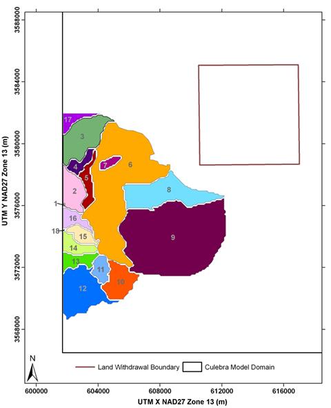
Figure TFIELD 2-10. Closed Drainage Sub-basins Identified in Southeastern Nash Draw. White areas are either outside Nash Draw or the study area.
Across the WIPP site, the Culebra can be considered confined, with little potential for direct vertical recharge for the relatively short time period covered in the WIPP Culebra model calibration (i.e., the length of multi-well pumping tests). Within portions of Nash Draw, the Culebra is very shallow (i.e., only covered by portions of the highly fractured Tamarisk) and observed water levels show the Culebra responds to precipitation events in a very short time (Appendix HYDRO-2014). Due to the interpretative nature of the confinement estimate, no numerical values of storativity were predicted from this geologic analysis, only zones of relatively higher or lower confinment, with an intermediate transition zone. The confined area has a relatively unambiguous definition, whereas the boundary between transition and unconfined is much more subjective.
The area of the Culebra considered confined (red in Figure TFIELD 2-11) is defined approximately by the interpreted margin of upper Salado halite dissolution (Powers et al. 2003). There is a significant increase in Culebra T values west and south of this margin, and this change is attributed to changes in fracture aperture associated with strain induced by dissolution. The transition zone (green in Figure TFIELD 2-11) includes areas where some data from wells indicate there is some vertical isolation of the Culebra, but information is less conclusive.
Most of the Culebra unconfined zone (blue in Figure TFIELD 2-11) is in central Nash Draw and out of the AP-114 Task 1 study area. The strategy for estimating relative Culebra confinement was to select areas where the Culebra is known or believed to be very shallow (≤30 meters (m) below ground surface) and where observed recharge points (caves, sinkholes, alluvial dolines) are believed to access units below the Magenta. Some large caves and sinkholes are developed in the Tamarisk gypsum beds and have a greater likelihood of providing hydraulic connection to the Culebra than similar openings in the Forty-niner gypsum beds. Many potash exploration holes within Nash Draw encountered lost-circulation zones, but the stratigraphic relationships of these zones to the Culebra are not well constrained. Thus, apart from the location from Livingston Ridge (the escarpment marking the eastern edge of the surface expression of Nash Draw) and the upper Salado dissolution margin, the factors determining confinement of the Culebra are generally qualitative.
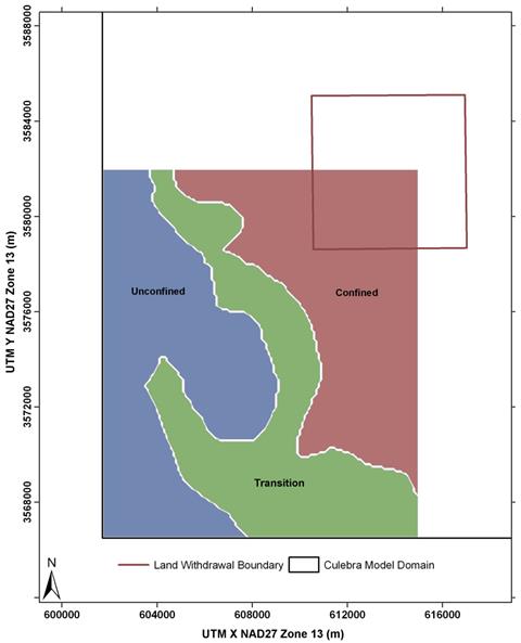
Figure TFIELD 2-11. Culebra Confinement Map for Southern Nash Draw Study Area. White areas are outside the Nash Draw geologic study area. Zones are shown over the entire model area in Figure TFIELD 5-3.
The amount of gypsum cements in fractures and vuggy porosity within the Culebra is believed to be inversely related to Culebra T (Beauheim and Holt 1990). They postulated gypsum fracture fillings limited Culebra T by closing fracture apertures, filling critical fracture junctions. The postulated relationship remained qualitative because too few well locations had both measured T values and describable core. Since 1990, the Culebra has been cored and hydraulically tested at 24 additional locations, providing sufficient data to construct a quantitative model linking Culebra T with the presence of gypsum cements. No soft data on gypsum cements was used in T-field construction or calibration before CRA-2009 PABC.
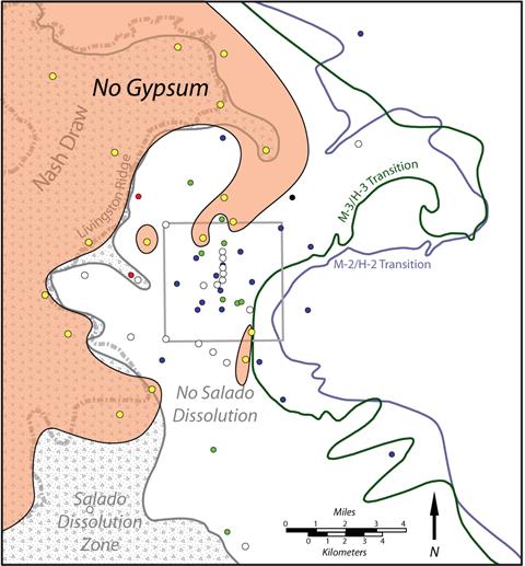
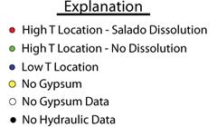
In Appendix F of Hart et al. (Hart et al. 2008), a simple quantitative model was constructed relating Culebra gypsum content to T. Using units defined by Holt (Holt 1997), maps were developed to illustrate spatial occurrence of gypsum in the Culebra. The maps used a gypsum index accounting for the relative Culebra gypsum content (Figure TFIELD 2-12 and Figure TFIELD 2-13). Using a critical value of the gypsum index, the high-T/low-T status of Culebra well locations were predicted with an accuracy >97% for WIPP well locations where both sufficient core and T estimates exist. These maps revealed that regions of no gypsum occur predominantly where Salado dissolution has affected the Culebra. The low-gypsum region in the southern WIPP LWB (Figure TFIELD 2-13) is similar to the high-diffusivity region defined by Beauheim (Beauheim 2007) (Figure TFIELD 4-2). Soft data were used to incorporate information about the influence of gypsum content on predicted Culebra T.
Figure TFIELD 2-12. Areas Where No Gypsum Has Been Found in Core Samples, Corresponding to a Greater Likelihood of Having Higher Culebra T Values
Figure TFIELD 2-13. Areas Where Wells Have Either No or Low Gypsum Content. The areas not shaded are likely to have high gypsum content and lower T.
The work outlined in Section TFIELD-3.0 was performed for CRA-2009 PABC under AP-114, Analysis Plan for Evaluation and Recalibration of Culebra Transmissivity Fields (Beauheim 2008), and still applies to CRA-2014. The conceptual model for base field creation was originally explained in Holt and Yarbrough (Holt and Yarbrough 2002), as Task 2, Subtask 1 of AP-088 for CRA-2004 PABC. Since then, the data supporting the conceptual model were updated and improved, but the model itself has changed very little. Any deviations of the CRA-2009 PABC model from the CRA-2009 model due to updates in data or process are discussed in this section. No updates have occurred for CRA-2014 since CRA-2009 PABC.
Figure TFIELD 2-2 illustrates the current geologic and hydrologic conceptual model of the Culebra dolomite in the vicinity of the WIPP site. Geologic controls on Culebra T were identified and a linear regression model relating these controls to T was constructed. The geology and geologic history of the Culebra has been described in detail elsewhere in the literature (Holt and Powers 1988; Beauheim and Holt 1990; Holt 1997). The following conceptual model was developed from this published work. Specifically, the model follows Holt (Holt 1997) in assuming variability in Culebra T is due strictly to post-depositional processes. Throughout the following discussion, the informal stratigraphic subdivisions of Holt and Powers (Powers 1988) are used to identify geologic units within the Rustler Formation, as listed in Figure TFIELD 2-3 and shown in map view for the Culebra model area in Figure TFIELD 2-8. The Culebra conceptual model given in this section passed a peer review (Burgess et al. 2008) before the calibration process in Section TFIELD-5.0 was begun.
It is hypothesized that Culebra T spatial distribution is a function of several geologic factors, some of which can be determined at a location using mapped geologic data, including:
1. Culebra overburden thickness,
2. fracture interconnection,
3. presence of gypsum cements in fractures and vuggy porosity,
4. dissolution of the upper Salado Formation below the Culebra, and
5. occurrence of halite in Rustler units above or below the Culebra.
High-T regions near the WIPP cannot be predicted using geologic data, as they represent areally persistent zones of well-interconnected fractures, and fracture interconnection cannot be observed or inferred from core or geophysical log data. Fracture interconnection is therefore treated as a stochastic process. Presence of gypsum cements in the Culebra, occurrence of Rustler halite, and Culebra overburden thickness instead varies slowly in space. These properties can be meaningfully mapped at the scale of the groundwater flow model.
The CRA-2009 PABC model domain was expanded to the east relative to the domain used for the CRA-2004 (U.S. DOE 2004) to reach an area where halite is present in all of the non-dolomite members of the Rustler Formation. This change was made to simplify the specification of the eastern boundary condition of the model. The current extent of the model domain is 601,700 to 630,000 m UTM X NAD27 and 3,566,500 to 3,597,100 m UTM Y NAD27. The domain was discretized into 100-m square cells, yielding a model 284 cells wide by 307 cells high. The Culebra was modeled as a single layer of uniform 7.75-m thickness (U.S. DOE 1996). The area covered by Figure TFIELD 2-8 corresponds to the model domain, showing the WIPP site boundary, the relevant geologic margins, and various Culebra monitoring wells. The model domain for CRA-2014 has not changed since CRA-2009 PABC.
An inverse relationship was hypothesized between Culebra overburden thickness and Culebra T. Overburden thickness is a metric for two different controls on Culebra T. First, fracture apertures can be related to overburden thickness (e.g., Currie and Nwachukwu 1974), as lower T are found where Culebra depths are greater (Beauheim and Holt 1990; Holt 1997). Second, erosion of overburden leads to stress-relief fractures, and the amount of Culebra fracturing increases as the overburden thickness decreases (Holt 1997). The structure contour map of Culebra elevation (Figure TFIELD 2-9) has been constructed using geophysical logs from hundreds of oil and gas wells, and geologic information from more than 100 WIPP-related boreholes. The difference between the land surface elevation (as obtained from U.S. Geological Survey (USGS) topographic maps) and Culebra elevation is the overburden thickness (Figure TFIELD 3-1). Culebra overburden thickness ranges from near zero in the southern end of Nash Draw, to over 550 m in the northeastern corner of Figure TFIELD 3-1. The depth to the Culebra from the land surface defined the value of d(x,y) for each cell in the Culebra model domain.
Figure TFIELD 3-1. Culebra Overburden Thickness Contours (m). Square is the WIPP LWB; irregular black outline west of WIPP is Nash Draw.
High-T zones within the Culebra are associated with interconnected fractures and occur randomly between areas bounded on the west by the Salado dissolution margin and on the east by H2 and/or H3 (the central area Zone 4 in Figure TFIELD 3-2). In these zones, fractures are well-interconnected, and fracture interconnectivity is controlled by a complicated history of fracturing with several episodes of cement precipitation and dissolution (Beauheim and Holt 1990; Holt 1997). Unfortunately, no geologic metric for fracture interconnectivity was identifiable in cores or from subsurface geophysical logs, and fracture interconnectivity has only been identified from in situ hydraulic test data.
Because of this lack of a corresponding easy-to-map geologic metric for fracture interconnectivity, the spatial location of high-T zones was considered to be a stochastic process that could not be predicted deterministically. The spatial layout of these zones was simulated for CRA-2009 PABC using geostatistical indicator kriging with conditioning data (this was not changed for CRA-2014 since CRA-2009 PABC). This stochastic development of zones was a change from CRA-2004 PABC (Holt and Yarbrough 2002), where the only conditioning information was based on the T at wells. Information was added to the geostatistical model to increase the likelihood of high T being placed between two wells that hydraulic testing has revealed to be associated with larger diffusivity values. North of the WIPP site (i.e., south of WIPP-30) evidence exists for both high levels of gypsum in the Culebra and relatively high D between pumping/observation well pairs. In this unique region, the geologic conceptual model indicates there is slightly lower probability of being in a high-T zone than in other areas where a high D or high T estimate exists. Section TFIELD-4.2 discussed the process of merging hydraulic hard and soft data (single-well T estimates and multi-well D estimates, respectively) with geologic soft data on gypsum.
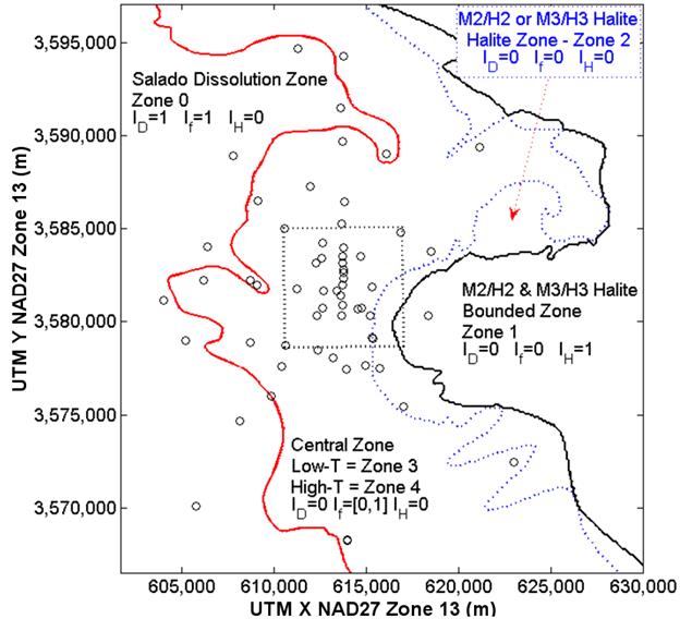
Figure TFIELD 3-2. Conceptual Model Zones With Indicator Values and Zone Numbers (Equation TFIELD 3.2). Zones 3 and 4 are distributed randomly between the Salado dissolution margin and westernmost M2/H3 or M3/H3 Rustler halite margins.
The Culebra T estimates at WIPP wells used in the CRA-2009 PABC modeling were the same as those used by Holt and Yarbrough (Holt and Yarbrough 2002), supplemented by more recent data reported from subsequent pumping tests (Roberts 2006 and 2007; Bowman and Roberts 2008). The log10
T data show a bimodal distribution in Figure TFIELD 3-3. Closely spaced wells sometimes show very different values; higher-T values are hypothesized to reflect the presence of well-interconnected fractures absent at lower-T locations. For example, wells WQSP-2 and WIPP-12 are only 454 m apart, but have T values differing by over two orders of magnitude (see blue star labeled W-12 and red circle labeled WQSP-2 in the north portion of the WIPP LWB in Figure TFIELD 2-8). Thus, the fractures present at WQSP-2 apparently do not extend to WIPP-12 or are not intersected by the WIPP-12 borehole. Well-interconnected fractures occur in regions affected by Salado dissolution (e.g., Nash Draw) and in areas with complicated cement dissolution and precipitation histories (e.g., high-T zones near the WIPP site). The natural break between the measured log10
T square meters per second (m2/s) values at −5.4 (Holt and Yarbrough 2002) is illustrated with a vertical black line in Figure TFIELD 3-3. The fracture-interconnection indicator (If
) is defined in terms of this break (Equation TFIELD 3.1).
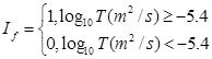 (TFIELD 3.1)
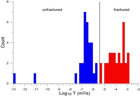
Figure TFIELD 3-3. Histogram of Log10 Culebra Transmissivity (T) Estimates at WIPP Wells from Single-well Tests
Slight modification was made to the Salado dissolution margin used in CRA-2009 PABC, compared to CRA-2009, as outlined in Section TFIELD-2.2.2. No modifications were made for CRA-2014 since CRA-2009 PABC. The indicator variable for Salado dissolution is ID
, and was defined to be 1 in areas of the model domain where dissolution has occurred, and 0 elsewhere. The Salado dissolution margin is plotted with the Rustler halite margins in Figure TFIELD 2-8.
The M2/H2 and M3/H3 Rustler halite margins were modified for CRA-2009 PABC compared to CRA-2009, as outlined in Section TFIELD-2.2.1. No modifications were made for CRA-2014 since CRA-2009 PABC. The margins are shown individually in Figure TFIELD 2-5 and Figure TFIELD 2-6, and together with the M1/H1 and M4/H4 Rustler halite margins and Salado dissolution margin in Figure TFIELD 2-8.
Wells SNL-6 and SNL-15 were drilled since Holt and Yarbrough (Holt and Yarbrough 2002). They are located east of the M2/H2 and M3/H3 halite margins, where halite is present in both intervals (see Figure TFIELD 2-8). As predicted by Holt (Holt 1997), the Culebra itself was partially cemented with halite at these locations, and estimated T were extremely low (Roberts 2007; Bowman and Roberts 2008). Based on these observations, Culebra T is assumed lower in the region where halite occurs both above (in the M3/H3 interval) and below (in the M2/H2 interval), than the Culebra T where halite occurs in only one of these intervals. The indicator term IH
was defined to be 1 at any point where halite is present in both the M2/H2 and M3/H3 margins, and to be 0 elsewhere.
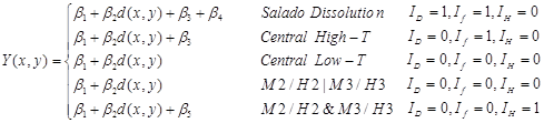
The following linear model for Y(x,y) = log10
T(x,y) was constructed
 (TFIELD 3.2)
where β
1 through β
5 are regression coefficients, the two-dimensional location vector (x,y) consists of NAD27 UTM Zone 13 x and y coordinates, d(x,y) is the Culebra overburden thickness (Figure TFIELD 3-1), If
is an indicator of whether interconnected fractures are present in the Culebra, ID
is the Salado dissolution indicator, and IH
is the halite bounding indicator. In this model, | means logical or, while & means logical and. Regression coefficient β
1 is the intercept value for the linear model. Coefficient β
2 is the slope of Y(x,y)/d(x,y). The coefficients β
3, β
4, and β
5 represent adjustments to the intercept for the occurrence of interconnected fractures, Salado dissolution, and halite bounding, respectively. Although other types of linear models could have been developed, Equation TFIELD 3.2 is consistent with the conceptual model relating Culebra T to geologic controls, can be tested using published WIPP geologic and T estimates, and can be potentially verified with new Culebra wells.
Because there are only two data points for T in the zone where Culebra is bounded by halite, and both are significantly lower than any other T values in the model, the β
5
IH
term in Equation TFIELD 3.2 was included to take into account the very low T zone. This was done to keep the conceptual model consistent for all zones, recognizing the base fields are primarily a starting point for subsequent calibration.
The combined results of the regression and the indicator kriging (Section TFIELD-4.3) were 1,000 base T-fields that shared certain geologic features, but were different from one another. This difference was provided by the stochastic placement of high-T areas in the central zone. These areas were placed using the GSLIB Sequential Indicator Simulation (SISIM) routine (qualified for use in WIPP PA according to NP 19-1 (Chavez 2006)). This routine used geostatistical methods to create stochastic indicator (Boolean value) fields.
The Culebra conceptual model given in this section passed peer review before proceeding with the CRA-2009 PABC calibration of the Culebra T fields (Burgess et al. 2008). The peer review panel found the methodology presented here to be adequate, accurate, and valid enough to justify proceeding with the numerical implementation and calibration of the Culebra T-fields. The panel found the CRA-2009 PABC conceptual model to be greatly improved, compared to the Culebra conceptual model used in the Compliance Certification Application (CCA) (U.S. DOE 1996). The panel found the understanding of the physical processes connecting the Culebra groundwater geochemistry with the Culebra hydraulic properties to be insufficient. The peer review panel did not feel this particular lack of understanding would be a problem in T-field development and calibration, due to the relatively high density of Culebra hydrologic data available at the WIPP site.
The work outlined in Section TFIELD-4.0 was performed under AP-114, Analysis Plan for Evaluation and Recalibration of Culebra T Fields (Beauheim 2008). This section discusses details associated with the incorporation of soft and hard data into the base T-field construction process. The base Culebra T-fields were the starting point for the calibration processes outlined in Section TFIELD-5.0. Aside from the definitions of some fixed parameter zones, all the parameters specified in the base T-field construction were allowed to be modified during the calibration process to produce model output that better matched observed steady-state and transient pressure observations. Inside the WIPP LWB there is a large amount of hard data to constrain the parameters of the groundwater model during calibration, while distant to the WIPP LWB the hard data are not sufficient to uniquely constrain the calibration. To help alleviate this problem, base T-field construction used soft data to provide additional constraints that could not be incorporated directly into the calibration process. Specification of soft data was used to create physically realistic starting points for the calibration. The starting point for the calibration has the most impact at locations distant to the WIPP LWB.
Kriging is a linear estimation process in the field of geostatistics that predicts an average value at locations without observations, using available observations and a model describing the variability of the function (i.e., the variogram, which is itself estimated from data). Indicator kriging is a specific form of the kriging where cutoffs are estimated (i.e., is the value above or below 1.0?), rather than a continuous value. Conditional stochastic simulation is a geostatistical approach for generating realizations that will have a common specified statistical structure specified through a variogram and data, but are otherwise random. Kriging predicts the mean and variance of a field, resulting in smooth mean fields. Kriging would be conceptually similar to generating many stochastic simulations and averaging the results. Conditional stochastic simulation with indicator kriging was used to predict location of high- and low-T areas
(is log10 T > −5.4 or < −5.4?), taking the model indicator variogram and various hard and soft data into account.
The constraints used to construct the base T-fields included a class-based linear regression relationship between log10
T and Culebra overburden within each type of well (see Section TFIELD-4.1) and geologic soft data such as the presence of halite in nearby units or gypsum cements in the Culebra (see Section TFIELD-4.2). The indicator variograms were constructed from these data (see Section TFIELD-4.3) and used to stochastically simulate the cutoff between high and low Culebra T (see Section TFIELD-4.4). The indicator kriging simulation result was a component of the base T-field construction (see Section TFIELD-4.5).
The best fit to estimate T from single well tests was based on a multi-line regression analysis. The wells were separated into three groups: wells in the Salado dissolution zone, wells with low-T pumping test results, and wells with high-T pumping test results. Figure TFIELD 4-1 shows the log10
T values from pumping test results, the Culebra overburden thickness, and the regression lines fit to each group's data individually. The cutoff between low and high log10
T is −5.4. Wells located where the Culebra is bounded above and below by halite (SNL-6 and SNL-15) were considered outliers and were not included in the regression analysis. Instead, the β
5
IH
term was chosen to yield values close to those interpreted from tests at SNL-6 and SNL-15 (presented in Appendix F of Hart et al. (Hart et al. 2008), Table F-1); this value was directly modified during the calibration stage in AP-114 Task 7 (Hart et al. 2009). The final regression equation for Y = log10
T (Equation TFIELD 4.1) and a table of the β values (Table TFIELD 4-1) resulted in a fit characterized by R
2 = 0.92 and F = 216.
 (TFIELD 4.1)
The remainder (ε) represents the misfit between the regression model and observed data.
Table TFIELD 4-1. β-values for Regression Equation TFIELD 4.1
|
β
1
|
β
2
|
β
3
|
β
4
|
β
5
|
|
−5.69805
|
−3.48357×10⁻³
|
2.06581
|
0.68589
|
−4.75095
|
The data and calculations were provided in Appendix A of Hart et al. (Hart et al. 2008).
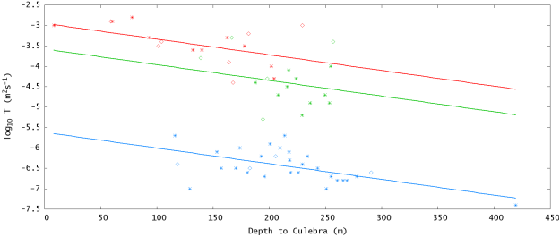
Figure TFIELD 4-1. Regression Lines for Low-T Wells (Blue), High-T and Non-dissolution Wells (Green), and Wells Within the Salado Dissolution Zone (Red). Open diamonds are wells new to the CRA-2009 PABC regression analysis (i.e., not included in CRA-2004 PABC).
Geologic and hydraulic information are included as soft data to maintain the geologic conceptual model through the stochastic indicator kriging simulations in Section TFIELD-4.4. Soft data define probabilities (P
low) a new well at a given point would have a low T value. For model cells that include wells where log10
T (m2/s) has been estimated from single-well hydraulic tests, the observation is referred to as hard data to distinguish it from more indirect contributions to T values associated with soft data. Model cells where hard data (single-well test-derived log10
T) is greater than −5.4 are assigned P
low = 0, while P
low = 1 for all cells containing low-T pumping test results. Estimated T used as hard data are presented in Table TFIELD 4-2, including coordinates, depth, and log10
T values used in regression model (from Listing A.1 of Appendix A in Hart et al. (Hart et al. 2008)).
Table TFIELD 4-2. Listing of Coordinates, Culebra Depth, and Log10
T Estimates from Single-well Tests (Hard Data) Used in Regression Model (Equation TFIELD 4.1)
|
Well
|
UTM X NAD27,
Zone 13 (m)
|
UTM Y NAD27,
Zone 13 (m)
|
depth to
Culebra (m)
|
log10
T
(m2/s)
|
|
H-10b
|
622975
|
3572473
|
419.25
|
−7.4
|
|
P-15
|
610624
|
3578747
|
129.24
|
−7.0
|
|
WIPP-12
|
613710
|
3583524
|
250.7
|
−7.0
|
|
AEC-7
|
621126
|
3589381
|
269.14
|
−6.8
|
|
H-15
|
615315
|
3581859
|
265.79
|
−6.8
|
|
WQSP-3
|
614686
|
3583518
|
260.38
|
−6.8
|
|
H-12
|
617023
|
3575452
|
254.97
|
−6.7
|
|
H-5c
|
616903
|
3584802
|
277.82
|
−6.7
|
|
WIPP-30
|
613721
|
3589701
|
195.69
|
−6.7
|
|
H-17
|
615718
|
3577513
|
219.03
|
−6.6
|
|
SNL-8
|
618523
|
3583783
|
291.5
|
−6.6
|
|
WIPP-21
|
613743
|
3582319
|
225.85
|
−6.6
|
|
WQSP-6
|
612605
|
3580736
|
180.31
|
−6.6
|
|
CB-1
|
613191
|
3578049
|
157.27
|
−6.5
|
|
H-14
|
612341
|
3580354
|
170.23
|
−6.5
|
|
SNL-10
|
611217
|
3581777
|
182.58
|
−6.5
|
|
WIPP-18
|
613735
|
3583179
|
243.08
|
−6.5
|
|
SNL-13
|
610394
|
3577600
|
118.26
|
−6.4
|
|
WIPP-22
|
613739
|
3582653
|
229.51
|
−6.4
|
|
ERDA-9
|
613696
|
3581958
|
218.08
|
−6.3
|
|
C-2737
|
613597
|
3581401
|
205.74
|
−6.2
|
|
H-2c
|
612666
|
3581668
|
192.94
|
−6.2
|
|
WIPP-19
|
613739
|
3582782
|
233.93
|
−6.2
|
|
H-16
|
613369
|
3582212
|
217.46
|
−6.1
|
|
H-4c
|
612406
|
3578499
|
153.31
|
−6.1
|
|
H-1
|
613423
|
3581684
|
209.55
|
−6.0
|
|
P-17
|
613926
|
3577466
|
173.89
|
−6.0
|
|
WQSP-5
|
613668
|
3580353
|
200.67
|
−5.9
|
|
D-268
|
608702
|
3578877
|
115.98
|
−5.7
|
|
H-18
|
612264
|
3583166
|
213.57
|
−5.7
|
|
SNL-5
|
611970
|
3587285
|
194.16
|
−5.3
|
|
H-19b0
|
614514
|
3580716
|
229.2
|
−5.2
|
|
DOE-1
|
615203
|
3580333
|
253.44
|
−4.9
|
|
WQSP-4
|
614728
|
3580766
|
236.42
|
−4.9
|
|
H-3b1
|
613729
|
3580895
|
207.87
|
−4.7
|
|
WQSP-2
|
613776
|
3583973
|
249.72
|
−4.7
|
|
WQSP-1
|
612561
|
3583427
|
215.79
|
−4.5
|
|
H-6c
|
610610
|
3584983
|
187.61
|
−4.4
|
|
SNL-9
|
608705
|
3582238
|
167.64
|
−4.4
|
|
Engle
|
614953
|
3567454
|
204.22
|
−4.3
|
|
H-11b4
|
615301
|
3579131
|
223.93
|
−4.3
|
|
SNL-14
|
614973
|
3577643
|
198.12
|
−4.3
|
|
WIPP-13
|
612644
|
3584247
|
217.17
|
−4.1
|
|
DOE-2
|
613683
|
3585294
|
254.51
|
−4.0
|
|
H-9c
|
613974
|
3568234
|
201.78
|
−4.0
|
|
SNL-18
|
613606
|
3591536
|
163.98
|
−3.9
|
|
SNL-2
|
609113
|
3586529
|
138.99
|
−3.8
|
|
WIPP-25
|
606385
|
3584028
|
140.06
|
−3.6
|
|
WIPP-28
|
611266
|
3594680
|
131.98
|
−3.6
|
|
P-14
|
609084
|
3581976
|
178
|
−3.5
|
|
SNL-17
|
609863
|
3576016
|
101.19
|
−3.5
|
|
SNL-19
|
607816
|
3588931
|
103.94
|
−3.4
|
|
WIPP-11
|
613791
|
3586475
|
256.95
|
−3.4
|
|
SNL-12
|
613210
|
3572728
|
166.73
|
−3.3
|
|
USGS-1
|
606462
|
3569459
|
162.44
|
−3.3
|
|
WIPP-27
|
604426
|
3593079
|
92.97
|
−3.3
|
|
SNL-1
|
613781
|
3594299
|
181.66
|
−3.2
|
|
SNL-3
|
616103
|
3589047
|
229.51
|
−3.0
|
|
WIPP-29
|
596981
|
3578694
|
8.23
|
−3.0
|
|
SNL-16
|
605265
|
3579037
|
58.83
|
−2.9
|
|
WIPP-26
|
604014
|
3581162
|
60.2
|
−2.9
|
|
H-7c
|
608095
|
3574640
|
77.88
|
−2.8
|
Two geologic margins, M2/H2 and M3/H3, were updated by Powers (2007a and 2007b), as summarized in Section TFIELD-2.2.1. Wells penetrating the Culebra in areas that are bounded both above and below by halite (e.g., SNL-6 and SNL-15) have been found to have very low T estimates, less than 10−11 m2/s (Roberts 2007). Wells bounded by only one margin (e.g., H-12 and H-17) have lower than average T estimates.
Because high-T fractures are not predicted where halite is present in the Rustler, model cells located on the combined M2/H2 and M3/H3 margin were assigned P
low = 1. This ensured that no high-T areas were placed on the boundary itself, largely a cosmetic consistency fix. Additionally, regression results for all model cells in the halite zone were replaced with values directly from the regression equation; indicator values were only used in Zones 3 and 4, and were not used east of the Rustler halite margins in Zone 1 (Figure TFIELD 3-2).
In all cases where sufficient core and T estimates exist, wells with no gypsum (Figure TFIELD 2-12) have high T, due to well-interconnected fractures. To account for this relationship, cells were assigned P
low = 0.05 where no gypsum is present. As seen in Figure TFIELD 2-12, this is a fairly large area. Rather than give all the cells in the area such a low P
low value, cells were selected from a regular grid at 1300-m spacing to receive soft data assignments (Figure TFIELD 4-3). A grid of 1300-m spacing was chosen to provide sufficient definition of the boundaries without overwhelming the SISIM geostatistical simulation with too many samples. The size of the matrix decomposed by SISM during estimation is proportional to the number of samples considered at each estimation location.
It was observed that in all cases where sufficient core and T estimates exist, wells outside of the low-gypsum region (Figure TFIELD 4-3) have low T because fracture interconnectivity is limited by gypsum cements. In the indicator kriging, areas outside of the low-gypsum region were assigned P
low = 0.95 to increase the likelihood of predicting low T in the simulation.
By definition, the areas of no-gypsum and high-gypsum content cannot overlap, therefore the high-gypsum data were sampled on the same grid used by the no-gypsum data. By using fractional likelihoods and sparse sampling, these soft data did not overwhelm the random sampling algorithm of SISIM and allowed for greater variation between base field realizations. The high/low-gypsum content map is shown in Figure TFIELD 2-13. The low-gypsum region was not sampled, since it overlapped the no-gypsum region. Instead, the high-gypsum region was used. The area of high gypsum directly north of the WIPP LWB was sampled at 300-m spacing, to compensate for the diffusivity soft data described in the next section and produce model results more similar to observed Culebra behavior during pumping tests.
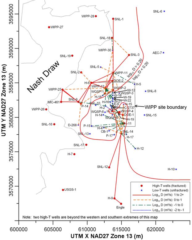
Figure TFIELD 4-2. Diffusivity Values Calculated Between Wells From Pumping Test Data. Connections where log10
D
> 0.2 are included as conditioning data with P
low = 0.25.
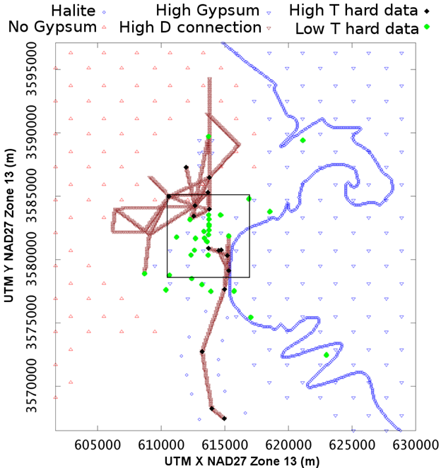
Figure TFIELD 4-3. Soft Data Points (Open Symbols) Generated During Step 2. Hard data points (filled symbols) are located at wells with single-well estimates of T. The black square is the WIPP LWB.
Soft data were used to incorporate the degree of hydraulic connection observed between pairs of wells (pumping and observation wells) into the construction of the base fields. The diffusivity D (m2/s) associated with the pumping and observation well pair was calculated from the results of many hydraulic tests conducted at the WIPP site (Beauheim 2007). A map of these values is shown in Figure TFIELD 4-2, showing colored lines connecting pumping and observation wells involved in the nine pumping tests used in T-field calibration (pumping/observation wells listed in Table TFIELD 5-2). The model cells falling on a straight line connecting two wells with a calculated log10
D > 0.2 (i.e., all red connecting lines and some orange dashed lines) were assigned P
low = 0.25 to account for the increased likelihood a cell on the connecting line would be high T (inverted maroon triangles in Figure TFIELD 4-3). Using P
low = 0 would have forced SISIM to create a direct path connecting two wells where a strong response to pumping was observed, and there is no geologic reason that these connections must be straight.
In addition to the high-T connection lines, a set of low-T points was placed roughly parallel to the SNL-14/SNL-12/H-9/Engle connection path to keep the high-T connection relatively narrow (blue circles in south central portion of Figure TFIELD 4-3). These points were assigned a P
low = 1, to ensure they would impact the indicator kriging simulation. Pumping SNL-14 in 2005 produced a strong response at H-9c nearly ten kilometers (km) to the south. During model development it was found the only way to recreate the observed response with the MODFLOW model was to incorporate a relatively narrow connecting zone of high T. Without adding some low-T points along the flanks of this path, SISIM tended to create a wide high-T area, which did not allow the drawdown response to propagate significantly from SNL-14 to H-9, as was observed. The observed response would be consistent with a narrow linear geological feature, which is difficult to simulate using the current MODFLOW model with 100-m grid spacing. These low-T points did not force the simulation to create a narrow high-T pathway in each realization, as many base fields still had large areas of high T that extend past these points. Fields generated with and without the narrow high-T pathway were modified through the calibration process, which included the SNL-14 pumping test data as calibration targets. This exercise was performed in an attempt to improve the ability of the base T fields to match observed data, since this might lead to fewer PEST iterations and quicker calibration times.
The final combined soft data field is shown in Figure TFIELD 4-3. The soft data input files and calculation scripts are provided in Appendix B of Hart et al. (Hart et al. 2008).
Single-well estimates of T are hard data shown on the figure with filled diamonds (data listed in Table TFIELD 4-2). Hard data are combined here with soft data in base T-field creation, but appear again (without soft data) as fixed pilot points in the T-field calibration process (Section TFIELD-5.0). Filled green diamonds are wells with log10
T estimates ≤ −5.4 (m2/s), and black filled diamonds are wells with log10
T estimates > −5.4 (m2/s).
The grid of inverted open blue triangles in the east indicate areas with "high gypsum" (white area in Figure TFIELD 2-13), while the grid of open red triangles in the west indicates areas with "no gypsum" (peach area in Figure TFIELD 2-12).
Lines of closely spaced inverted brown triangles represent the connections between pumping and observation wells interpreted with a log10 diffusivity (D) > 0.2 m2/s, including all solid red and some dashed orange lines in Figure TFIELD 4-2.
The open blue circles ("Halite" in the figure legend) are used in two ways to enforce high probability for low T in two different locations. The first use is the line of closely spaced open blue circles corresponding to M2/H2 or M3/H3; locations east of this line have either halite above or below the Culebra. This boundary marks the eastern edge of the random placement of high-T and low-T zones (Zones 3 and 4 in Figure TFIELD 3-2). The second group, the open blue circles straddling the line connecting Engle, H-9, SNL-12, and SNL-14 (running south to north from the bottom middle of the figure), represents a low-T zone added to increase the contrast of the high-T zone along this line of south-to-north connectors, to better represent results observed in the SNL-14 multi-well pumping test.
The geostatistical indicator simulations done as part of the base T-field development are only utilized in the central section of the model domain, between the Salado dissolution area to the west and the low-T halite-sandwiched region to the east. Therefore, only wells in this middle section are used for construction of the indicator variogram. A total of 46 wells that provide information regarding log10
T were used in the calculation of the indicator variograms. The indicator value is determined by comparing each log10
T value to a threshold log10
T value,
Tt
= −5.4,
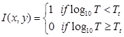 (TFIELD 4.2)
Where I(x,y) denotes the unitless indicator value at well location (x,y). The experimental indicator variogram was fit with a spherical variogram model, whose model parameters are given in Table TFIELD 4-3. Figure TFIELD 4-4 illustrates the experimental and model indicator variograms. The proportion of low-T values in the data set is 0.652. The variance of an indicator value is (1 − p)p, where p is the proportion of high or low values. The variance for these indicator data is 0.227 and is used directly as the sill in the variogram modeling (dashed horizontal line in Figure TFIELD 4-4). The parameters in Table TFIELD 4-3 are used as input to the SISIM program for creation of the stochastic component of the base T-fields. In an attempt to identify anisotropy, model variograms were calculated in both the NE-SW and NW-SE directions (see Appendix C of Hart et al. (Hart et al. 2008)). These directional variograms analyses were inconclusive, only omnidirectional (i.e., isotropic) variograms were used in the final analysis.
Table TFIELD 4-3. Variogram Parameters for Isotropic Fit to Indicator Data Variogram. Omnidirectional variogram calculated with a lag spacing of 500 m.
|
Parameter
|
Value
|
|
Model Type
|
Spherical
|
|
Nugget
|
0.0
|
|
Sill
|
0.227
|
|
Range
|
2195 m
|
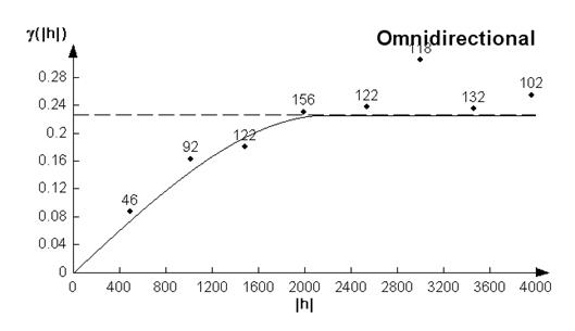
Figure TFIELD 4-4. Experimental Variogram (Dots) and Spherical Model (Line) for Indicator Values. x-axis is lag distance [meters], y-axis is the unitless indicator; numbers by dots indicate the number of pairs represented at each lag.
With previous sections describing the indicator variogram model, hard T data values, and soft geologic and hydrologic data, stochastic realizations of high-T zones were constructed using the GSLIB program SISIM (Deutsch and Journel 1998). An example indicator field is given in Figure TFIELD 4-5. Maps summarizing statistics for the 1,000 resulting base T-fields are presented in Figure TFIELD 4-6 and Figure TFIELD 4-7. These figures show the impact the conditioning information had on the overall fields. The combined M2/H2 and M3/H3 margins have a standard deviation of 0 and are constant at the proper value as desired. Areas designated as higher likelihood of high T do show an average value that trends towards the high-T value (in this case, 0), but they still have a standard deviation that is non-zero, indicating that there is some variability in those areas. The same is true in areas outside the low-gypsum region. Additionally, areas with no conditioning information have higher standard deviations, indicating that high-T zone placement in those locations was allowed to be fully variable. Though there are some visible artifacts from the grids used in the average and standard deviation fields (locations of soft data points in Figure TFIELD 4-3 are discernible in Figure TFIELD 4-6 and Figure TFIELD 4-7), the individual realizations, such as Figure TFIELD 4-5, do not show these artifacts. Additionally, the majority of the artifacts occur outside the central zone, which is the only place the indicator fields are used. The indicator fields created by this process are the best possible combination of hydraulic and geologic conditioning given current data.
There is a relatively high density of hard data available inside the WIPP LWB, which significantly constrains the estimation process there. Geostatistical simulation is most useful to fill in large gaps near the edges of the model domain where a small number of observations exist. It must also be considered that these base-T fields are just a first guess for the model calibration process, which utilizes the single-well T and both the steady-state and multi-well pumping test drawdown data as calibration targets. Ultimately, these data drive the calibration, adjusting input parameters to better match observed data. See Section TFIELD-5.4 for figures and discussion illustrating the extent to which the input fields were adjusted to match the data (e.g., see Figure TFIELD 5-19).
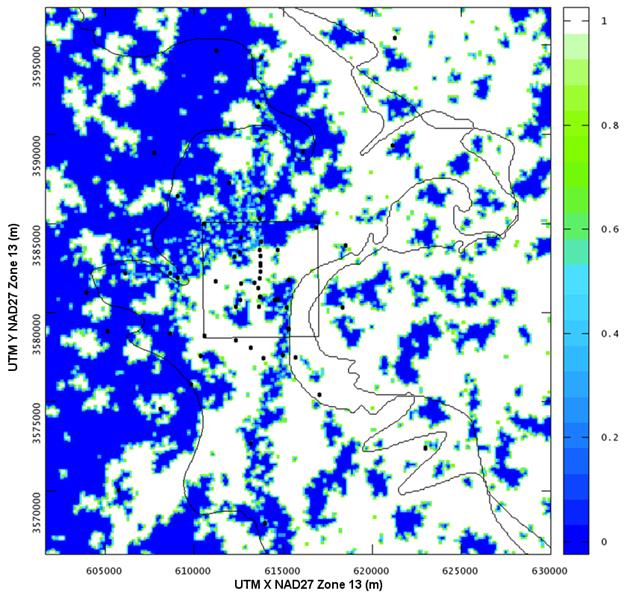
Figure TFIELD 4-5. Sample Indicator Field for Realization r123. 1 indicates low T and 0 indicates high T.
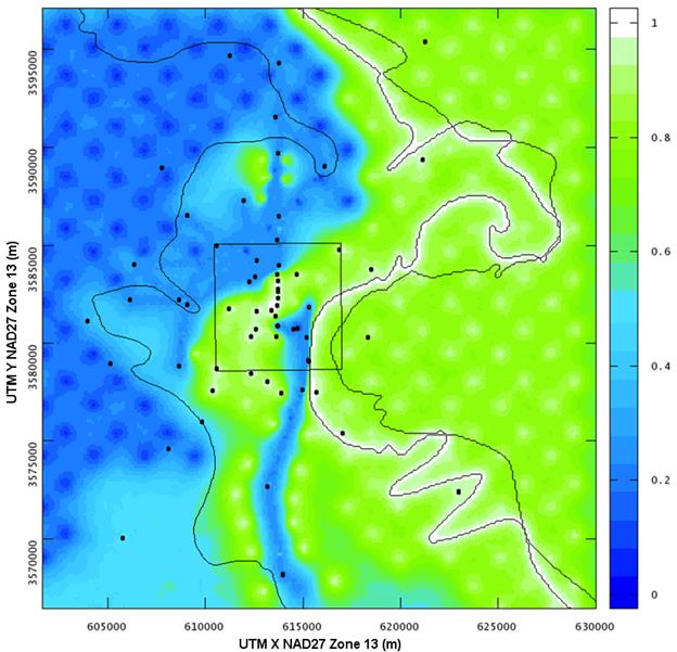
Figure TFIELD 4-6. Average Indicator Values Across All 1000 Base Realizations. 1 indicates low T and 0 indicates high T.
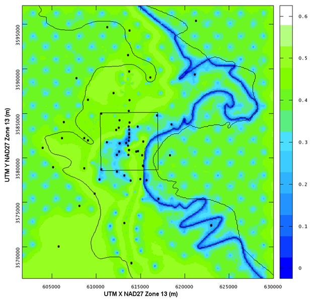
Figure TFIELD 4-7. Standard Deviation of Indicator Values Across All 1000 Base Realizations
Once the indicator fields were created, the T values were assigned using Equation TFIELD 4.1 using a Perl script. Equation TFIELD 4.3 was used to calculate Y = log10
T at each cell,
Y(x,y) =
b
[Z(x,y)] +
a
[Z(x,y)] d(x,y) (TFIELD 4.3)
where
b
and
a
represent combinations of the β-coefficient based on the zone (Z(x,y)) of the cell. Table TFIELD 4-4 shows how the variables in the original linear regression equation (Equation TFIELD 4.1) were related to Equation TFIELD 4.3. Figure TFIELD 3-2 shows the indicator zone distribution.
Table TFIELD 4-4. Correlation of β and I Values from Equation TFIELD 4.1 to a and b Values in Equation TFIELD 4.3
|
|
Zone 0
Salado
|
Zone 1
Halite 2
|
Zone 2
Halite
|
Zone 3
Central low T
|
Zone 4
Central high T
|
|
If
|
1
|
0
|
0
|
0
|
1
|
|
ID
|
1
|
0
|
0
|
0
|
0
|
|
IH
|
0
|
1
|
0
|
0
|
0
|
|
Ih
|
0
|
1
|
1
|
0
|
0
|
|
b
|
β
1 + β
3 + β
4
|
β
1 + β
5
|
β
1
|
β
1
|
β
1 + β
3
|
|
a
|
β
2
|
β
2
|
β
2
|
β
2
|
β
2
|
The Perl script was executed on all 1,000 realizations. A sample final base T field is presented in Figure TFIELD 4-8 for realization r123 (a random representative selection from the possible fields). The mean log10
T-field across all 1,000 realizations is presented in Figure TFIELD 4-9. The standard deviation of log10
T is presented in Figure TFIELD 4-10. Very low standard deviation occurs across the 1000 base realizations outside the stochastically sampled areas, including the higher T areas to the west and the lower T areas to the east (Figure TFIELD 4-10). These stochastically sampled areas are the main source of variability between the 1000 base realizations. The variability of the indicator variable across the realizations (Figure TFIELD 4-7) is one component of the variability observed in the final T values in the base T fields (plotted normalized to the range {0,1} in Figure TFIELD 4-10). The regression analysis produced variability in the predicted T values in a zone related to the variability in the overburden thickness.
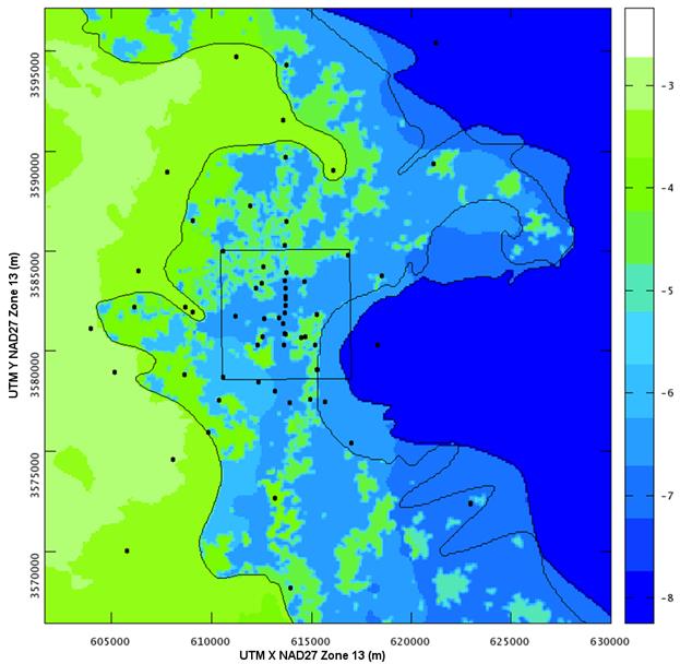
Figure TFIELD 4-8. Sample Log10
T (m2/s) Base Field Realization r123

Figure TFIELD 4-9. Mean Log10
T (m2/s) Values Across All 1000 Base Realizations
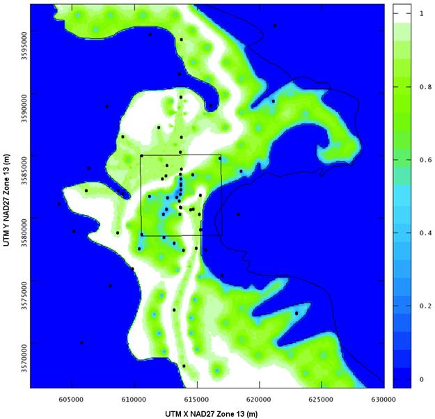
Figure TFIELD 4-10. Normalized Standard Deviation of Log10
T (m2/s) Values Across All 1000 Base Realizations
The work outlined in Section TFIELD-5.0 was performed under AP-114, Analysis Plan for Evaluation and Recalibration of Culebra T Fields (Beauheim 2008). The calibration of the T-fields used 200 of the 1,000 base fields from the results of AP-114 Task 5 (Hart et al. 2008, summarized in Section TFIELD-4.0) as starting points for the calibration process. More than 200 fields could not be calibrated, due to time constraints. Calibration is the process of systematically adjusting the input parameters to the MODFLOW model (fields of T, A, S, and R) to reduce the sum of the squared differences between field observations and MODFLOW model output (steady-state and transient head).
The pilot point calibration method was implemented using the parameter estimation software PEST. Automatic model calibration was utilized to make the process more easily documentable and reproducible, compared to manual calibration (i.e., trial and error). The MODFLOW model used to simulate groundwater flow through the Culebra contains a large number of active model cells for T, A, and S fields. Estimating each model element independently would require estimating hundreds of thousands of unknown parameters. The pilot point approach makes the calibration process more tractable by lowering the number of parameters to estimate. Instead of estimating each parameter in each model cell independently, parameter values are estimated at strategically placed pilot point locations. Parameter values at each model cell are then interpolated from the pilot points using kriging as a pre-processing step between parameter assignment by PEST and MODFLOW model execution. The pilot point approach allows mixing estimated and fixed pilot points (e.g., T pilot points at wells with single-well hydraulic test estimates of T). The pilot point approach was also used in CRA-2004 PABC and a variant of it was used (without PEST) in the CCA. Both steady-state and transient head calibration targets are discussed in Section TFIELD-5.1. The parameter zones, pilot point locations for each parameter, initial conditions, and boundary conditions are specified in Section TFIELD-5.2. The components of the MODFLOW model used with PEST, and the utilities required to pre-process and post-process the inputs and outputs from the model during the calibration are discussed in Section TFIELD-5.3. Finally, some post-calibration analysis of the results is presented in Section TFIELD-5.4.
The initial T values at pilot points were taken from the base fields. In addition to T, the horizontal T anisotropy (A), the storativity (S), and a linear section of recharge (R) were also calibrated. The same zone definitions used for developing the base T fields (see TFIELD-4.0) were used for T pilot points (although zone numbers changed), and similar zone definitions were used for anisotropy. Zones for storativity and recharge were based on other analyses completed in the area surrounding the WIPP site (see Section TFIELD-5.2.1). Pilot points were selected for each parameter and initial values were selected that were consistent with the conceptual model used to create the base fields (see Section TFIELD-5.2.2 and Section TFIELD-5.2.7).
A model variogram for T was created using the estimated T from single-well hydraulic tests. This variogram was also used for all parameters, as it was the only one that could be created from field data (see Section TFIELD-5.2.8). This variogram was used to create kriging factors that were then used to create continuous fields from the pilot point values. The T, A, S, and R fields were then used as inputs to the MODFLOW numerical model to produce simulated head and drawdown results (see Section TFIELD-5.2.10).
Once the MODFLOW models produced simulated drawdown and head results, the modeled results were compared to the field data for the tests that were modeled. The residual of an observation is calculated in PEST as the weighted difference between measured and modeled data. Observation weights were selected to make the sum of the weighted steady-state head errors approximately equal to the sum of errors of four observation wells in a transient pumping test to approximately balance the steady-state and transient model-to-data misfits. The PEST optimization uses a single objective function, which is the sum of the steady-state and transient residuals. Because the improvement of model fit for steady-state heads might come at the expense of fit to transient pumping tests, a decision was made to balance the importance of the two groups in the calibration effort. The residuals were used by PEST to construct a finite-difference approximation of the Jacobian matrix. The Jacobian matrix is a measure of the sensitivity each model prediction has to each adjustable parameter, and is used to optimize the pilot point parameter values. The goal of the optimization is to minimize the objective function value, a measure of the misfit between model predictions and observed data (see Section TFIELD-5.2.9).
Because traditional construction of the Jacobian matrix requires at least Np
+ 1 forward model calls (Np
parameters estimated in the calibration), using 1,100-plus parameters would be impossible without additional efficiency in the optimization. The PEST singular value decomposition (SVD) assist approach reduces the size of the Jacobian matrix by only using the most significant "super-parameters" that correspond to the eigenvectors with the largest singular values, estimated using the SVD of the Jacobian matrix. The SVD process required initial calculation of a full Jacobian matrix, but then reduced the subsequent number of required forward calls by a factor of four to six. The result was that three calls to PEST were required to calibrate the fields (see Figure TFIELD 5-1):
1. a single full Jacobian calculation, which required 1,100+ forward model calls;
2. an SVD calibration using the reduced parameter set that ran up to 50 iterations, requiring between 100 and 400 forward model calls per iteration; and
3. a final PEST run with the best parameter results to create the final fields corresponding to the best parameter values calculated during the SVD-assisted calibration.
Total calibration time for a single base field was approximately seven days using six processors (one master node and five slave nodes).
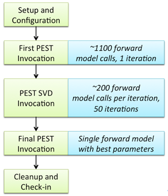
Figure TFIELD 5-1. Complete Calibration Process for a Single Realization
After approximately 140 fields had been calibrated, a few steady-state calibration targets were found to be incorrect by several meters. A total of 150 fields were calibrated using the incorrect targets, and an additional 50 fields were started using the corrected heads (Beauheim 2009; Johnson 2009a and Johnson 2009b). To deal with the incorrect values, a limited recalibration was performed on the results of the first 150 calibrations (see Section TFIELD-5.3.2). The same process that has been described was followed for the limited secondary calibration, but since the initial parameter values were taken from the calibrated results, only the necessary pilot point locations near the updated steady-state head values were allowed to be changed, and the SVD portion of the PEST recalibration was limited to 10 iterations. The end result was 200 fields, with 150 of these fields having undergone a secondary calibration to incorporate corrected field observation data. The impact of this change is discussed in Section TFIELD-5.3.3.
The end result of the calibration was the first 200 of the original 1,000 field sets (T, A, S, and R) calibrated to one set of steady-state heads and nine transient, multi-observation well pumping tests. More than 200 of the 1,000 base T-fields could not be calibrated due to time constraints associated with the calibration effort. Since the 1,000 base T-fields were generated randomly, the first 200 were in effect a random sample. The 100 best-calibrated fields (those with the smallest residuals) were selected as the final results from this task (see Section TFIELD-5.3.4). Several statistical analyses were performed on the fields themselves to generate average values and variances in the field results (Section TFIELD-5.4.1).
The complete calibrations were performed under quality-assurance run control with inputs and outputs stored in a version control repository on a central server. The calibrations required approximately six months of continuous runtime on a total of 80 processors. See Hart et al. (Hart et al. 2009) for details.
Two sets of head values were used for calibration of the Culebra flow model. The first dataset consists of 42 freshwater head values measured in May 2007, which were used as steady-state calibration targets (see Table TFIELD 5-1 for values used and see Johnson (Johnson 2009a and Johnson 2009b) for details). Appendix HYDRO-2014 shows the behavior of water levels in wells since 2007. The data in Appendix HYDRO-2014 support the continued use of 2007 water levels to represent steady-state conditions at the WIPP up to the CRA-2014 (see additional discussion in Appendix HYDRO-2014). The second dataset consists of drawdown data collected during 9 independent multi-well pumping tests conducted over a span of more than 20 years (see Table TFIELD 5-2 for lists of observation wells and relevant references).
The steady-state MODFLOW simulation is calibrated against data in Table TFIELD 5-1. Each of the nine transient pumping tests in Table TFIELD 5-2 are simulated as a separate MODFLOW model simulation. A "single" forward model run actually involved 10 individual MODFLOW simulations (1 steady-state and 9 transient simulations), each using the same input parameter fields, but different pumping configurations. Some wells appeared in multiple pumping tests (e.g., H-15, H-18, or ERDA-9). These wells had calibration targets associated with multiple transient forward simulations. The MODFLOW model is discussed more in Section TFIELD-5.2.10.
SNL-6 and SNL-15 are listed as steady-state targets in Table TFIELD 5-1, but they are located in the constant-head portion of the model domain and therefore their corresponding model-predicted values are not adjustable through changes in the T field.
Table TFIELD 5-1. Freshwater Head Observations Used as Steady-state Calibration Targets
|
Well Name
|
May 2007
head target (m AMSL)
|
|
C-2737
|
921.23
|
|
ERDA-9
|
924.88
|
|
H-2b2
|
929.62
|
|
H-3b2
|
918.68
|
|
H-4b
|
916.34
|
|
H-5b
|
939.12
|
|
H-6b
|
936.44
|
|
H-7b1
|
914.58
|
|
H-9c
|
912.8
|
|
H-10c
|
922.02
|
|
H-11b4
|
917.09
|
|
H-12
|
916.53
|
|
H-15
|
920.32
|
|
H-17
|
916.24
|
|
H-19b0
|
918.84
|
|
IMC-461
|
928.95
|
|
SNL-1
|
941.86
|
|
SNL-2
|
937.65
|
|
SNL-3
|
939.81
|
|
SNL-5
|
938.59
|
|
SNL-6
|
1110
|
|
SNL-8
|
929.94
|
|
SNL-9
|
932.05
|
|
SNL-10
|
931.54
|
|
SNL-12
|
915.24
|
|
SNL-13
|
918.19
|
|
SNL-14
|
916.33
|
|
SNL-15
|
1060
|
|
SNL-16
|
918.68
|
|
SNL-17A
|
916.78
|
|
SNL-18
|
939.87
|
|
SNL-19
|
937.58
|
|
USGS-4
|
911.11
|
|
WIPP-11
|
940.65
|
|
WIPP-13
|
939.78
|
|
WIPP-19
|
933.66
|
|
WIPP-25
|
937.57
|
|
WIPP-30
|
939.37
|
|
WQSP-1
|
938.28
|
|
WQSP-2
|
939.87
|
|
WQSP-3
|
936.43
|
|
WQSP-4
|
919.5
|
|
WQSP-5
|
918.18
|
|
WQSP-6
|
921.96
|
Table TFIELD 5-2. Summary of Transient Observations Used as Calibration Targets
|
Pumping Well(s)
|
Observation Wells1
|
Total # obs.
|
Reference
|
|
WQSP-2
|
H-18, DOE-2, WQSP-1, WIPP-13
|
77
|
Beauheim and Ruskauff 1998
|
|
H-19 and H-11
|
WQSP-5, H-1, H-15, DOE-1, ERDA-9, WIPP-21, H-3b2
|
143
|
Beauheim and Ruskauff 1998
|
|
WQSP-1
|
H-18, WIPP-13
|
36
|
Beauheim and Ruskauff 1998
|
|
WIPP-11
|
WQSP-2, WQSP-3, WIPP-12, SNL-9, SNL-5, H-6b, SNL-3, SNL-2, SNL-1, WIPP-30, WQSP-1, WIPP-13
|
250
|
Toll and Johnson 2006b; Roberts 2006
|
|
H-11
|
H-4b, H-12, H-14, H-15, H-17, DOE-1, CB-1, P-15, P-17, H-3b2
|
130
|
Beauheim 1989
|
|
WIPP-13
|
WIPP-19, WIPP-18, H-2b2, H-6b, WIPP-12, WIPP-25, DOE-2, WIPP-30, P-14
|
167
|
Beauheim 1987b
|
|
SNL-14
|
H-9c, H-4b, SNL-13, SNL-12, H-15,
H-17, C-2737, ERDA-9, H-19b0,
H-3b2, H-7, H-11b4
|
252
|
Toll and Johnson 2006a; Roberts 2006
|
|
P-14
|
D-268, H-18, WIPP-26, H-6b, WIPP-25
|
82
|
Beauheim and Ruskauff 1998
|
|
H-3
|
DOE-1, H-2b2, H-1, H-11b2
|
69
|
Beauheim 1987a
|
|
1.
1
See Figure TFIELD 4-2 for locations
of pumping and observation wells and diffusivity values estimated from pumping tests.
|
This step comprised the setup and configuration processes that were the same for every calibrated base field. Step 1 included the creation and definition of zones for each of the parameters and the selection of pilot point locations and initial values. Because of the stochastic nature of the transmissivity fields, unique zones are associated with each field, as defined in Hart et al. (Hart et al. 2008). The process to set up each field was the same, but certain elements, such as the exact number of pilot point locations used, were unique to each field.
The model domain and extent are identical to the domain defined in Section TFIELD-3.1. The base T-fields were taken from the results of Section TFIELD-4.5. Some model input files were created statically, and were used for every calibration. Some model input files were created dynamically for each calibration, but used the same variables and parameters in their creation.
Parameter zones were defined for each of the calibrated parameters. These zones or regions were defined to be consistent with the conceptual model for Culebra flow defined in Hart et al. (Hart et al. 2008) and summarized in Section TFIELD-3.0. The parameter zones were chosen to organize common pilot points groups together in the PEST calibration. Numerical values of parameter zones (i.e., zone numbers) are often different from those used in the conceptual model. Figure TFIELD 2-8 shows the different margins that define geologic zones and the locations of the Culebra wells that have been drilled in the vicinity of the WIPP.
The T zones were defined to be consistent with the zones used in the geologic model and soft data analysis (Section TFIELD-4.2). As shown in Figure TFIELD 5-2, a high-T zone exists to the west (zone 2), corresponding to the area of Salado dissolution, and a mixture of higher and lower T values corresponding to the stochastic zones (zone 0 and 1) provided in the base fields defined the center of the model domain. Unlike AP-114 Task 5 (Section TFIELD-4.5), where it was a separate zone, the area between the H2/M2 and H3/M3 margins (green in Figure TFIELD 5-2) was included in the same zone (zone 1) as the lower T stochastic areas provided by the base fields. The area east of both the H2/M2 and H3/M3 margins - where the Culebra is bounded both above and below by halite-cemented elements - was defined to be its own zone (zone 3), as was done in AP-114 Task 5. A no-flow boundary roughly follows the axis of Nash Draw defining the final region (zone 4), which is inactive and applies to all parameters.
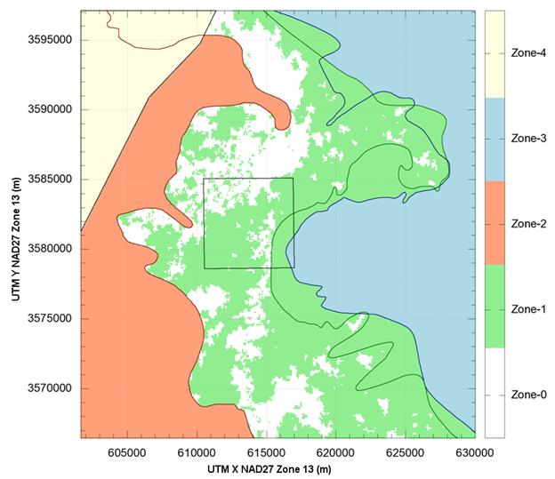
Figure TFIELD 5-2. Transmissivity Zone Map for a Single Realization. Zones 0 and 1 are the stochastic zones created in Hart et al. (2008); Zone 2 is the high-T Salado dissolution area; Zone 3 is the very low-T halite-bounded area; Zone 4 is the northwestern inactive area.
The T anisotropy field used the same zones defined for T. The T values in the north-south (y) direction were calculated by multiplying the transmissivity value for the east-west (x) direction (given in the T-field) by the anisotropy value (A) at a given cell
T
NS = T
EW
A. (TFIELD 5.1)
The map shown in Figure TFIELD 5-2 represents the zonation used for both A and T.
Besides the no-flow area (zone 4), four zones were defined for storativity estimation. The westernmost region (zone 2) is unconfined, as described in Powers et al. (Powers et al. 2006) (summarized in Section TFIELD-2.3.2). The largest area (zone 0) is fully confined, with its western boundary roughly following the Salado dissolution margin. The area between these two regions (zone 1) is the transition zone, where the Culebra is uncertainly confined. As with the T and A zones, the area east of both the H2/M2 and H3/M3 margins is a separate region (zone 3), but in this case storativity is simply held constant at the initial confined-zone value. A map of the storativity zones is shown in Figure TFIELD 5-3.
The unconfined zone was implemented as a zone of high confined storativity to simplify the numerical model by approximating the non-linear unconfined problem with a linear storativity one. By defining a much higher storativity value in the unconfined part of the domain, unconfined behavior can be approximately modeled using a confined numerical model, which is linear and executes quicker than the unconfined non-linear model. Since the unconfined or transition zone does not exist inside the WIPP LWB, this choice has little impact on interpretation of transient hydraulic tests there, and this choice has no impact on steady-state flow simulations (S is only used in transient simulations) used to predict radionuclide transport in PA.
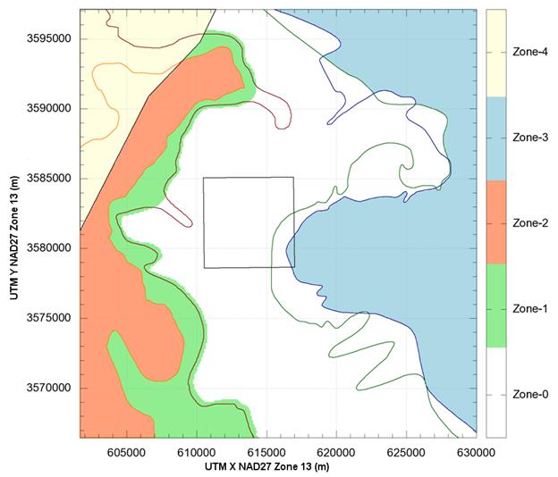
Figure TFIELD 5-3. Storativity Zones. Zone 0 is confined; Zone 1 is a transition between confined and unconfined; Zone 2 is unconfined; Zone 3 is confined and uncalibrated from the initial confined value; Zone 4 is inactive (no flow).
The conceptual model presented in Holt (Holt 1997) and Hart et al. (Hart et al. 2008) indicates that a groundwater divide exists somewhere southwest of the WIPP site. Previously in CRA-2004 PABC and CRA-2009, this groundwater divide was represented by extending the no-flow zone all the way to the southern boundary (McKenna and Hart 2003). Because the model used in this current task included the unconfined zone, it was decided to model the groundwater divide using recharge instead of a no-flow boundary. The areas of possible recharge were defined in AP-114 Task 1B (Powers 2006), summarized in Section TFIELD-2.3.1. Recharge values had to be extremely small (on the order of 10−11 m/s) to ensure convergence of steady-state MODFLOW simulations. Rather than try to determine which of the configurations presented in Task 1B was the "best" approximation, a similar simple approximation to the older no-flow approach was used. A recharge zone consisting of a line of cells extending NW to SE along the axis of the largest topographic feature (and roughly following the old no-flow boundary from McKenna and Hart (McKenna and Hart 2003) was used as the recharge zone. See Figure TFIELD 5-4 for a map of the recharge zone.
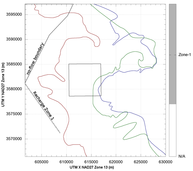
Figure TFIELD 5-4. Zone 1, the Zone of Non-zero Recharge. Zone 1 is the linear feature directed southeast from the center of the west edge of the model domain. The remaining model area has no recharge.
While the boundary conditions were not variable parameters in the calibration, the definition of the specified-head boundary conditions was an important part of the setup and configuration step. The no-flow zone in the northwest was defined to be the same as was used in AP-088 for CRA-2004 PABC. Though the T in this area is extremely low (10−13 to 10−11 m2/s), there should be some flow exiting along the zone margin, however minute. Testing at SNL-6 and SNL-15 indicates that the hydraulic heads in this area may be recovering ultimately to levels above the land surface (Roberts 2007; Bowman and Roberts 2008; Appendix HYDRO-2014, Section 7.1
). The "halite-sandwiched" zone east of either M2/H2 or M3/H3 was simultaneously made extremely low T and set to fixed-head values at the ground surface elevation. While this meant that the head values at SNL-6 and SNL-15 were no longer estimable, it was considered the simplest way to model the nearly stationary nature of the water in this zone using MODFLOW-2000. The flow zones are shown in Figure TFIELD 5-5, and the selection of the initial values is discussed in Section TFIELD-5.2.7. The northern, western, and southern flow boundaries were all fixed-head boundaries.
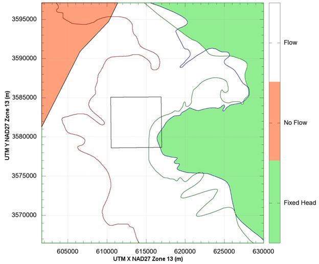
Figure TFIELD 5-5. Flow Zones. The fixed-head zone is green; the no-flow zone is salmon; the white area is normal flow. The fixed-head zone includes one cell along the northern, southern, and western boundaries.
Once the zones were defined, pilot point locations were selected. There were two types of pilot points, fixed and variable, and two placement approaches, gridded and linear. Selection of the points for each parameter required a combination of both types and approaches. The exact algorithm used to calculate placement is detailed in Hart et al. (Hart et al.2009), and resulted in the pilot point locations used and shown in Figure TFIELD 5-6 through Figure TFIELD 5-9.
In addition to pumping test wells, extra pilot points were placed in the transmissivity fields. These were included along the northern and southern boundaries to try to limit the effects that the fixed-head boundaries would have on transient pumping and the steady-state model results. The estimated T values from single-well pumping and slug tests were used as fixed T points that corresponded to the tested wells (see Table TFIELD 4-2 for test-derived transmissivity values). See Table TFIELD 5-3 for the ranges of pilot point values used, and see Figure TFIELD 5-6 for pilot point locations.
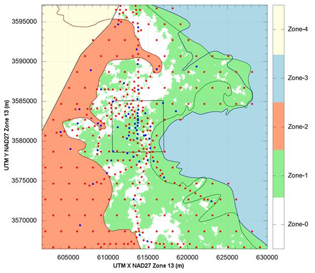
Figure TFIELD 5-6. Transmissivity Pilot Point Locations. Blue points are fixed values and red points are variable parameters. Zones correspond to a single realization.
Table TFIELD 5-3. Initial Values of Parameters at Pilot Points
|
Parameter
|
Zone
|
log10 Value1
|
Pilot Point log10 Calibration Limits
|
|
Transmissivity
|
Zone 0
|
−0.003484 d(x,y) − 3.6322
|
[−19.0,−1.0]
|
|
Zone 1
|
−0.003484 d(x,y) − 5.6981
|
[−19.0,−1.0]
|
|
Zone 2
|
−0.003484 d(x,y) − 2.9463
|
[−19.0,−1.0]
|
|
Zone 3
|
−0.003484 d(x,y) − 10.4490
|
[−19.0,−1.0]
|
|
Anisotropy
|
All Zones
|
0.0
|
[ −0.5, 0.5]
|
|
Storativity
|
Zone 0
|
−5.0
|
[ −5.5,−4.5]
|
|
Zone 1
|
−4.0
|
[ −6.0,−0.5]
|
|
Zone 2
|
−1.5
|
[ −2.5,−0.5]
|
|
Zone 3
|
−5.0
|
Fixed
|
|
Recharge
|
Zone 1
|
−11.0
|
[−19.0,−1.0]
|
|
1
d(x,y) is Culebra overburden thickness.
|
Anisotropy was unique because no fixed values and therefore no fixed pilot points were used. This result is due to the single-well tests not providing any estimate of anisotropy, and the multi-well tests providing too localized an estimate of anisotropy (only valid for a single cell or two in the model). See Figure TFIELD 5-7 for the locations of anisotropy pilot points.
The only variable storativity pilot points in the confined zone were along straight lines connecting pumping and observation wells in transient pumping tests. The gridded points were set as fixed values, since it was assumed there was no information allowing for effective calculation of storativity outside the transient tests. All pilot points located within the unconfined and transition zones were defined as variable. See Figure TFIELD 5-8 for the location of storativity pilot points.
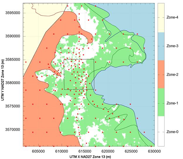
Figure TFIELD 5-7. Anisotropy Pilot Point Locations. All anisotropy pilot points were variable parameters. Zones correspond to a single realization.
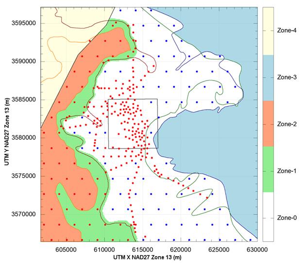
Figure TFIELD 5-8. Storativity Pilot Point Locations. Only pilot points along lines between wells in transient pumping tests and points in the unconfined zones (zones 1 and 2) were variable (red dots); the remaining pilot points were fixed (blue dots).
Because the recharge zone was a line, only four pilot points were needed in the entire zone. In this case, the pilot point nearest the western domain boundary was set as a fixed value of
10−30 m/s, which was interpreted as zero by the pre-processors to MODFLOW, and the other three were variable. See Figure TFIELD 5-9 for the location of the recharge pilot points.
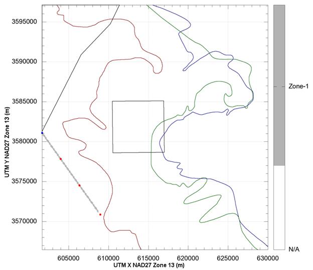
Figure TFIELD 5-9. Recharge Pilot Point Locations. The pilot point along the model domain boundary was fixed, while the other three points were variable.
Section TFIELD-5.2.7.1 discusses the initial values assigned to parameters before calibration, while TFIELD-5.2.7.2 discusses the assignment of a head field to the initial condition and certain specified-head boundary conditions in the groundwater flow model.
The initial values for each of the pilot points were defined according to the conceptual model and the values presented in Hart et al. (Hart et al. 2008), and summarized in Section TFIELD-3.0. For T, this meant that the same equation used to create the base T fields was used to define the initial values for the pilot points, based on their zone. Anisotropy was set to isotropic conditions (A = 1) for all points. Storativity was defined to start at 10−5 for the confined zone (the same value that was used for S in CRA-2004 PABC model AP-088), at 10−4 in the transition zone, and at 10−1.5 in the unconfined zone. Recharge was initialized as 10−11 m/s, a value found to be sufficiently small to allow MODFLOW to perform an initial run prior to PEST calibration. The zone-by-zone initial values for each parameter, and the limits placed on the range the values could take in calibration, are presented in Table TFIELD 5-3.
See Table TFIELD 4-2 for fixed T values.
Initial heads (H
0) were created using a multivariate equation based on normalized x and y coordinates (-1 ≤ {x,y} ≤ +1). The equation was designed to keep head along the northern boundary just above the measured head at SNL-1 and head along the southern boundary below the level measured at H-9c. These constraints were the defining factors on the constants in the equation that follows. This process was done only once, and the result was used as a static input file for all calibrations. The field was defined by the following equations
 (TFIELD 5.2)
where sign() is the sign of its argument (either +1 or -1) and |y| is absolute value. For values east of both the H2/M2 and H3/M3 boundaries, the ground-surface elevation was used as the initial head value; see Appendix A of Hart et al. (Hart et al. 2009) for details. The resulting initial head field is shown in Figure TFIELD 5-10.
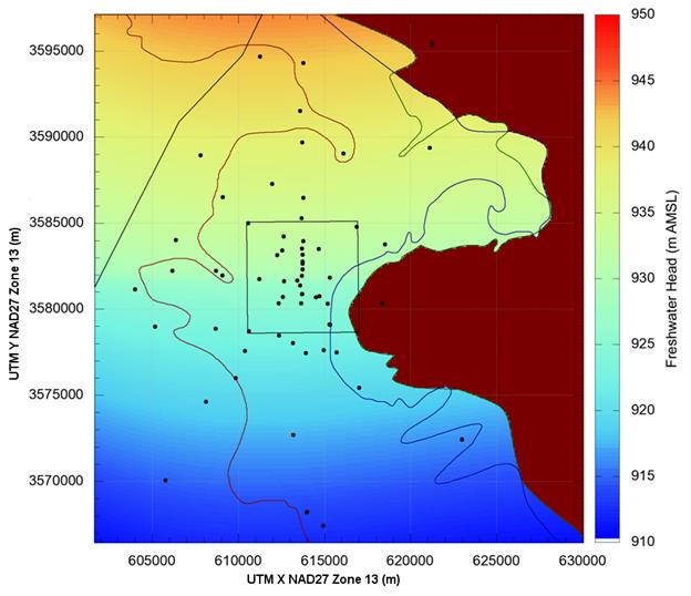
Figure TFIELD 5-10. Initial Head Values for Use in MODFLOW Steady-state Solution. Brick red head values were fixed at the ground surface elevation (>1,000 m AMSL).
Transmissivity fields are created from pilot points using kriging. Some pilot points are adjusted using PEST, while other pilot points are held fixed, because they correspond to estimated T values at wells with pumping tests. A variogram is needed to interpolate and extrapolate from the pilot points onto every element of the MODFLOW grid.
The transmissivity variogram (different from the indicator kriging variogram discussed in Section TFIELD-4.3) was created using transmissivity values estimated from well tests at 62 of the wells around the WIPP site. Wells outside the model domain and values at SNL-6 and SNL-15 were excluded from the calculation. The values at SNL-6 and SNL-15 are both several orders of magnitude lower than at the other wells, and are in a geologically distinct zone. While initial calculations showed that there was some statistical anisotropy, there were not sufficient measurements to create an anisotropic variogram. The complete steps for creating the variogram are presented in Hart et al. (Hart et al. 2009), Appendix B. The final parameters used are shown in Table TFIELD 5-4.
Table TFIELD 5-4. Parameters for T Model Variogram, Fitted to Transmissivity Data Using an Omnidirectional Variogram with Lag Spacing of 1,500 m
|
Parameter
|
Value
|
|
Model Type
|
Exponential
|
|
Nugget
|
0.02 (log10
T)2
|
|
Sill
|
1.95 (log10
T)2
|
|
Range
|
9,500 meters
|
The observations (steady-state freshwater heads and pumping test drawdowns) used as calibration targets for PEST are summarized in Section TFIELD-5.1. Residuals are calculated as the difference between measured and model-generated freshwater heads or drawdowns. The PEST utility program MOD2OBS is used to extract the observations from model output at times and locations associated with each steady and transient observation.
Inverse modeling (i.e., automatic calibration) requires a numerical model which generates results to compare against observed information. In this task, a MODFLOW 2000 (Harbaugh et al. 2000) flow model was developed for the Culebra that could use the base fields generated in Hart et al. (Hart et al. 2008) as inputs. As was done in CRA-2004 PABC (McKenna and Hart 2003), the link algebraic multi-grid (Mehl 2001) solver was used to increase speed and performance compared to other available solvers. In addition to T, it was decided to calibrate the local horizontal T anisotropy, storativity, and a strip zone of recharge as parameters in the calibration. Having these four parameters - T, A, S, and R - required a slightly more complex MODFLOW model implementation than was used in CRA-2004 PABC AP-088 (McKenna and Hart 2003). Specifically, both storativity and anisotropy were single values previously, and changing these to cell-by-cell values required the use of the layer property flow package instead of the block centered flow package used previously. Using recharge also required the addition of the recharge package; both packages are part of the standard MODFLOW distribution (Harbaugh et al. 2000). For the known information, steady-state heads from 2007 and drawdown results from nine different pumping tests performed between 1985 and 2008 were used as the measured data. A conceptual diagram of the MODFLOW model with its inputs and outputs is shown in Figure TFIELD 5-11.
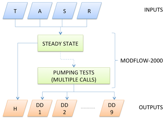
Figure TFIELD 5-11. Flow Chart Showing the Forward Model Used In the Model Calibration. T, A, S, and R are parameter fields. H represents the steady-state flow solution. DD
1-DD
9 represent transient drawdown computed for the 9 individual pumping tests from 9 separate forward simulations.
The calibration process used multiple forward model calls to evaluate the impact that perturbing an input parameter has on model predictions at locations and times corresponding to observations. This process was computationally intensive, and involved 80 processors on 2 different computing clusters running for 6 months to calibrate 200 of the 1,000 base T fields.
The calibration process was done using the PEST inverse modeling software suite and its groundwater utilities. The steps involved in each forward model run during the PEST calibration are illustrated in Figure TFIELD 5-12; the complete calibration process is shown in Figure TFIELD 5-1.
The completed PEST simulation included the creation of the fields from the kriging factors and pilot points (PPK2FAC, FAC2REAL, REAL2MOD), the MODFLOW calls, and finally the observation extraction utilities (MOD2OBS and OBS2REAL), which extract modeled cell head or drawdown values from a binary MODFLOW output file. For SVD iterations, another preprocessor, PARCALC, is used to create the pilot point values from the super parameters (i.e., eigenvectors related to the largest eigenvalues - see description in TFIELD-5.0). The model script (model.sh), the REAL2MOD script, and the OBS2REAL script were written for this task, and are included in Appendix G of Hart et al. (Hart et al. 2009). PPK2FAC, FAC2REAL, and MOD2OBS are PEST utilities.
The first call to the PEST program was a single outer iteration to estimate the Jacobian matrix. This required over 1,100 forward model calls, one for each variable parameter value. Once the Jacobian matrix was calculated, the SVDAPREP program decomposed the Jacobian matrix into eigenvectors and kept the super parameters corresponding to the largest singular values. The result was a set of 100 to 300 super parameters that were then used with a 50-iteration PEST calibration. The termination criteria were:
- a maximum of 50 iterations,
- three successive iterations without an improvement in the objective function, or
- a relative decrease of less than 0.001 in the objective function for three iterations.
Once termination criteria had been reached, the PEST program would output the best parameters to a file. This file was then used to create one final PEST control file, which issued a single model run with the best parameters as input. The results of this final call were then used to calculate the measures of fit and the final fields.
The run control details regarding the calibration process are presented in Appendix G of Hart et al. (Hart et al. 2009). Using the ReadScript.py run control system allowed automatic check-out of input files, execution, and check-in of the results to version control following calibration.
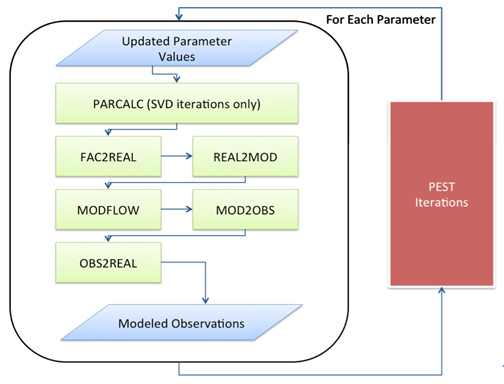
Figure TFIELD 5-12. Flowchart Illustrating the PEST Calibration Process
Because some of the original steady-state calibration targets were incorrect, the fields that had already been calibrated to the incorrect data needed to be recalibrated to the new data. The two wells with the most significant changes, ERDA-9 and SNL-8, had more than one meter change from the old to new values. At ERDA-9 the calibrations had consistently been unable to match the incorrect head value, which was too low compared to the higher corrected value. Without any recalibration, correcting the value for ERDA-9 produced better model fits.
The new calibration target for SNL-8 was based on a recalculation of the freshwater head (Johnson 2009a and Johnson 2009b). Because SNL-8 was not an observation well in any of the transient pumping tests, and because it was to the east and upgradient from the WIPP LWB, only a section of the fields were recalibrated to correct for the change in the calibration target at SNL-8. It was hoped that this would allow the T, S, A and R fields to change to match the SNL-8 head without requiring the week-long recalibration for each of the affected fields if the entire domain was recalibrated.
The recalibration process involved fixing all the parameters that had previously been calibrated, except for those parameters in a rectangular area around and upgradient from SNL-8. The complete area definition was 14 km east-west by 9 km north-south with the southwest corner at 616000 m X, 3580000 m Y UTM NAD27, and is shown in red on Figure TFIELD 5-13. All other aspects of the automatic calibration, including the forward model and the SVD assist process, were left the same. The resulting fields had significantly better fits to the steady-state heads, and little impact was seen on the transient test results (Table TFIELD 5-5).
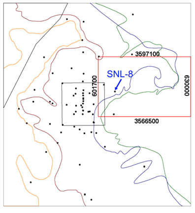
Figure TFIELD 5-13. Recalibration Boundary Shown in Red To the Northeast of the WIPP Site. Recalibration boundary limits are UTM X and Y NAD27 Zone 13 (m).
After examination of the acceptance criteria (discussed in the next section), some fields were recalibrated again, using the same recalibration process but holding none of the parameter values fixed at previously calculated values. This process essentially added some additional calibration iterations to these fields. This was only done on 15 fields that were now completely within the acceptance criteria for steady-state heads, and just outside the acceptance criteria for transient tests (Table TFIELD 5-5). The intent of this additional calibration was to increase the quality of the transient fits to get a total of 100 fields that met both the steady-state and transient calibration requirements. This secondary recalibration process was continued until 100 fields were obtained that met the requirements, and it did not always improve fits (i.e., in some cases the fields were already as fully calibrated, given the number of pilot points and observations and initial conditions).
Table TFIELD 5-5. Summary of Statistics Regarding Average Steady-state and Transient Errors Across Three Calibration Groups
|
|
Steady-state
Average Error (cm)
|
Pumping Response
Average Error (cm)
|
|
|
|
Minimum
|
Average
|
Maximum
|
Minimum
|
Average
|
Maximum
|
n
|
|
A
|
45.6
|
68.9
|
195.0
|
12.9
|
16.4
|
34.2
|
135
|
|
B
|
50.5
|
73.8
|
115.3
|
12.5
|
16.5
|
23.0
|
50
|
|
C
|
57.8
|
66.1
|
72.8
|
13.9
|
15.4
|
17.4
|
15
|
|
A: Realizations with targeted recalibration near SNL-8.
B: Realizations with correct SNL-8 data.
C: Realizations recalibrated twice.
|
Because some fields were calibrated only once (set B: 50 fields following correction of the steady-state values), some fields were calibrated once and then underwent a localized recalibration (set A: the 135 first fields calibrated), and some fields even underwent a second round of calibration (set C: 15 fields), the impact this may have had on the final selection of fields was evaluated. Summaries of statistics for these calibration groups are given in Table TFIELD 5-5, while Appendix E of Hart et al. (Hart et al. 2009) contains the complete list of fields.
Because the final selection process did not look at which set of fields the results were taken from, the mix of fields should be similar to a random selection if the calibration processes were producing equivalent results. The random selection of fields from set B can be modeled as a binomial distribution with the p-value of 0.25 and n = 100. If the results are within the 95% confidence interval for a random selection of fields, then there should be between 17 and 33 fields selected from the set B. The final results used 83 fields from sets A and C, and the remaining 17 were selected from set B. This is within the confidence interval, so it is concluded that the different processes had no impact on the selection of the final fields. The selection of fields from set C versus those from set A can be modeled the same way, with a p-value of 0.10 and n = 83. The final selection included 10 from set C, which is within the confidence interval of 3 to 13 fields, and again the calibration process did not impact the field selection.
Because this mix of final fields is acceptable and came strictly from the cutoff values, and not from any deliberate attempt to select from one group or another, all 100 fields meeting the acceptance criteria are equally good and equally probable representations of the Culebra.
The selection criteria for the "best" calibrated fields consisted of comparing the absolute error of the modeled steady-state heads (sum of absolute values of residuals between model and data) to a cutoff value, and comparing the absolute average error of the modeled transient responses (sum of absolute values of errors at individual observation wells averaged through time) to a cutoff value. The steady-state and transient criteria were evaluated separately, and only fields that were less than the cutoff value for both sets of tests were selected as the final fields. The final cutoff values used were the mean value of the errors taken across all 200 fields, and are presented in Table TFIELD 5-6. The cutoffs were selected to choose approximately half of the fields. Using the mean values resulted in a set of 102 fields, so the two fields with the largest sum of the two metrics were discarded. In Figure TFIELD 5-14, the sum of the steady-state average errors was graphed against the sum of the transient pumping tests' average errors, and the selected and unselected fields are shown. The trend line shows graphically how PEST allows tradeoffs while keeping the improvement in errors as balanced as possible. The final field IDs are presented in Table TFIELD 5-7.
Table TFIELD 5-6. Cutoff Values for Final Field Selection
|
Test Type
|
Average Error Selection Cutoff
|
|
Steady State
|
0.699 m
|
|
Transient Pumping Response
|
0.164 m
|
Table TFIELD 5-7. Final Selected Field Identifiers
|
r001
|
r055
|
r207
|
r652
|
|
r002
|
r058
|
r256
|
r655
|
|
r004
|
r059
|
r260
|
r657
|
|
r006
|
r060
|
r273
|
r664
|
|
r007
|
r061
|
r276
|
r669
|
|
r009
|
r064
|
r279
|
r694
|
|
r010
|
r070
|
r298
|
r707
|
|
r012
|
r073
|
r327
|
r727
|
|
r013
|
r074
|
r328
|
r752
|
|
r017
|
r076
|
r361
|
r791
|
|
r024
|
r078
|
r431
|
r806
|
|
r027
|
r082
|
r440
|
r808
|
|
r028
|
r083
|
r465
|
r809
|
|
r029
|
r084
|
r486
|
r814
|
|
r032
|
r090
|
r489
|
r823
|
|
r034
|
r092
|
r506
|
r861
|
|
r037
|
r095
|
r508
|
r883
|
|
r038
|
r097
|
r511
|
r902
|
|
r040
|
r098
|
r515
|
r910
|
|
r041
|
r102
|
r522
|
r921
|
|
r045
|
r104
|
r568
|
r922
|
|
r051
|
r137
|
r571
|
r940
|
|
r052
|
r142
|
r631
|
r981
|
|
r053
|
r191
|
r634
|
r982
|
|
r054
|
r203
|
r640
|
r984
|
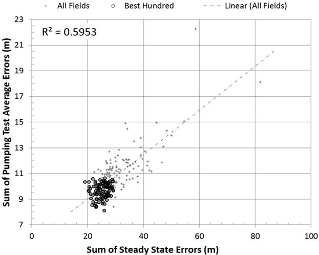
Figure TFIELD 5-14. Selection of Best Fields From All Fields by Weighted Sum of Steady-state Errors and Sum of Average Pumping Test Average Errors
The post-calibration analysis consisted of performing statistical analyses on the selected fields, and examining the calibrated forward model outputs. The full results of the steady-state forward model outputs are presented in Appendix C of AP-114 Task 7 (Hart et al. 2009), pumping test results are presented in Appendix D, and tabular results are presented in Appendix E of the same report. Calibrated model inputs and outputs for the 100 selected fields are presented in Attachment A to Appendix TFIELD.
Plots of mean and standard deviation of the final 100 fields are given in Section TFIELD-5.4.1.1. The bulk T of the final calibrated fields are also compared to the bulk T of the base fields, using membership in the high or low T categories. Similarly, Sections TFIELD-5.4.1.2
and TFIELD-5.4.1.3 show summary statistics regarding the calibrated S and R fields, respectively.
The T values presented in this section are the effective T values (T
e), which include A. Effective transmissivity was calculated as
log10
T
e = log10
T
EW + ½ log10
A (TFIELD 5.3)
which is the average of log10T in the north-south and east-west directions (see Equation TFIELD 5.1 in Section TFIELD-5.2.1.2). The bulk T
e, which is the average log10
T
e value of all cells in a given zone or zones, was calculated for the central and Salado dissolution region (zones 0-2) and compared to the bulk T
e of the same zones from the base fields. The eastern, very low-T region (zone 3) was compared separately. The bulk T
e values are shown in Table TFIELD 5-8. The mean effective T
e and the standard deviation of T
e are presented in map form in Figure TFIELD 5-15 and Figure TFIELD 5-16. The mean effective transmissivity map does not show the very low T zone east of the halite margins to improve the colormap contrast across the area around the WIPP site.
Because pilot point parameter values were essentially unconstrained for T (they were allowed to change across 18 orders of magnitude as shown in Table TFIELD 5-3), some areas in zones 0 and 1 could change from a low-T zone into the range generally considered high-T and vice versa. The defining value for high-T was set in AP-114 Task 5 (Hart et al. 2008) to be the bulk transmissivity value of the base fields: −5.41 log10 m2/s. At each cell, the number of fields whose initial and final T values were in the high-T zone was calculated, and the maps of those numbers for the base and calibrated fields are presented in Figure TFIELD 5-17 and Figure TFIELD 5-18, respectively. The total number of fields where transmissivity effectively changed zones is represented graphically in Figure TFIELD 5-19 and Figure TFIELD 5-20. In these figures, the white regions define areas where no fields changed groups. The two measures shown in these sets of maps provide an indication of how the geologically based conceptual model used to create the base fields was altered by the steady-state and transient hydraulic information.
Table TFIELD 5-8. Bulk Log10
T
e Values Comparison
|
Base field bulk log10
T
e
(Zones 0-2)
|
−5.41 log10 (m2/s)
|
|
Calibrated field bulk log10
T
e
(Zones 0-2)
|
−5.02 log10 (m2/s)
|
|
Base field bulk log10
T
e
(Zone 3)
|
−11.74 log10 (m2/s)
|
|
Calibrated field bulk log10
T
e
(Zone 3)
|
−10.47 log10 (m2/s)
|
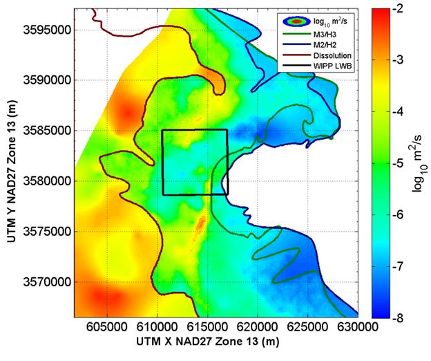
Figure TFIELD 5-15. Mean Effective Transmissivity (T
e) for Zones 0-2 Across the 100 Final Selected Fields. All 100 calibrated T
e fields are plotted in Appendix TFIELD Attachment A.
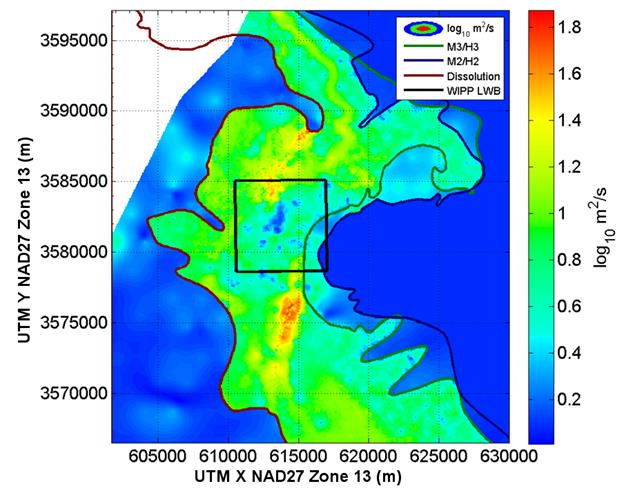
Figure TFIELD 5-16. Standard Deviation of Effective Transmissivity (T
e) for All Zones Across the 100 Final Selected Fields. All 100 calibrated T
e fields are plotted in Appendix TFIELD Attachment A.
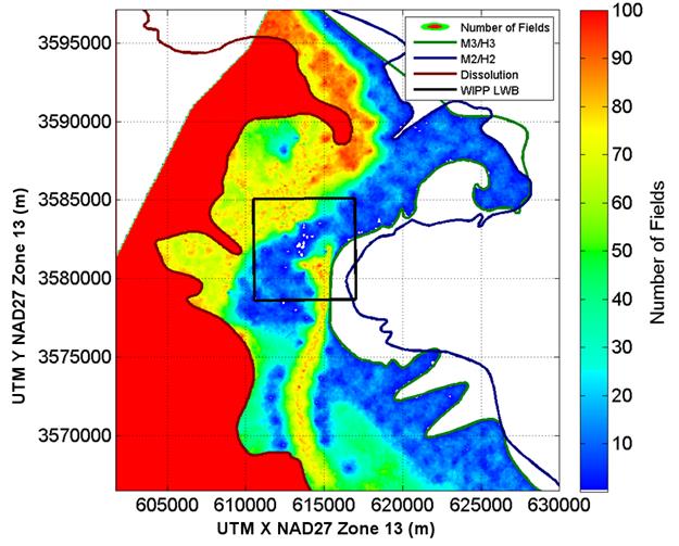
Figure TFIELD 5-17. High-T Zone Membership Calculated for the Base 100 T Fields Corresponding to the 100 Selected Calibrated Fields
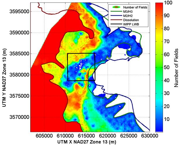
Figure TFIELD 5-18. High-T Zone Membership Calculated for the Calibrated T Values
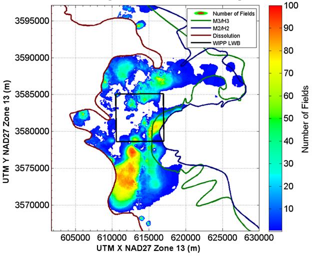
Figure TFIELD 5-19. Number of T Fields Where Low T Became High T Through PEST Calibration
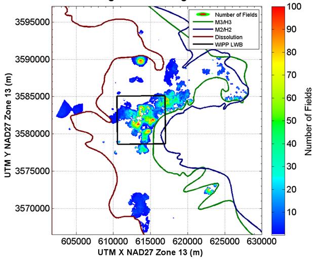
Figure TFIELD 5-20. Number of T Fields Where High T Became Low T Through PEST Calibration
The mean and standard deviation of the final S fields are presented in Figure TFIELD 5-21 and Figure TFIELD 5-22. The mean S fields indicate that the overall S values in the confined and transitional zones did not change much from their initial values. Figure TFIELD 5-22 highlights the area northwest of P-14 with a red dashed oval. This area has high variability in estimated S across the 100 selected realizations. This may have some relation to the relatively poorer fits of the transient data for the WIPP-25 response to the P-14 pumping test in the model.
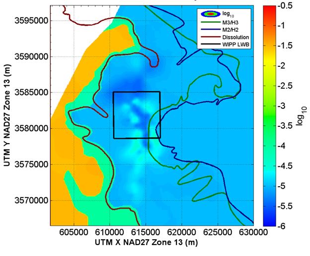
Figure TFIELD 5-21. Mean Storativity Values Across the 100 Final Calibrated Fields. Individual S fields are plotted in Appendix TFIELD Attachment A.

Figure TFIELD 5-22. Standard Deviation of Storativity Values Across the 100 Final Calibrated Fields. Red oval shows P-14 to WIPP-25 area of influence. Individual S fields are plotted in Appendix TFIELD Attachment A.
The final recharge values were all less than the initial values of 10−11 m/s (3.2 × 10⁻⁴ meters per year (m/yr)). Compared to the other parameters, there was very little change in recharge. Because the recharge zone was linear, in addition to the cell-by-cell mapping, a view of the average, minimum and maximum recharge values is shown as a cross section in the cross-direction (across a row) as if looking from the south to the north through the domain in Figure TFIELD 5-23.
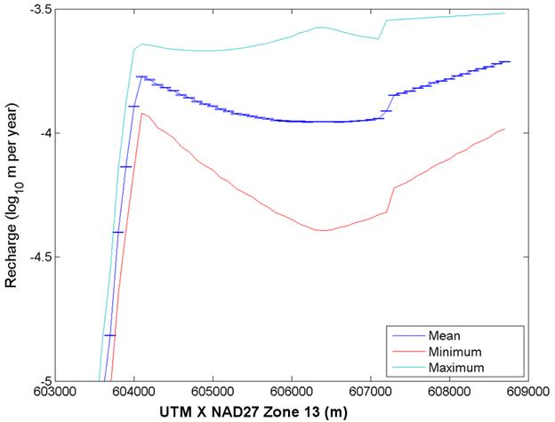
Figure TFIELD 5-23. Recharge as Viewed Through Columns From the South. The initial value was set at 10−3.5 m/year. The sharp dropoff to the west is the transition to the single fixed-recharge point of 10−11.5 m/year (interpreted as zero by REAL2MOD).
The two main divisions of the results are the steady-state head results and the pumping test results. The results presented here only represent the 100 final selected fields, and therefore the maximum error is limited by the selection criteria described in Section TFIELD-5.3.4: an average steady-state error of less than 0.699 m and an average pumping test observation error of less than 0.164 m.
Figure TFIELD 5-24 shows the modeled steady-state head values plotted against the measured head values. The one-to-one correspondence line shows the ideal match, and the modeled results are presented as box-and-whisker plots at each observation well. Figure TFIELD 5-25 shows all 4,200 head errors across all 100 fields as a histogram of error values for steady-state head. Additional figures and tables summarizing steady-state calibration are presented in Appendix C of Hart et al. (Hart et al. 2009). The model-measurement misfit can be modeled as a zero-mean Gaussian distribution with a standard deviation of 0.10 m (McKenna and Wahi 2006). The measurement error distribution curve is included in Figure TFIELD 5-25.
Graphs for each of the transient pumping test results are presented in Appendix D of Hart et al. (2009). The average value of the error in the final fields ranged from 0.12 m to 0.164 m across all tests, with an average error of 0.15 m. The maximum error for a single observation well ranged from 0.005 m to 2.5 m, with an average of 0.36 m as the maximum error at a given observation well.
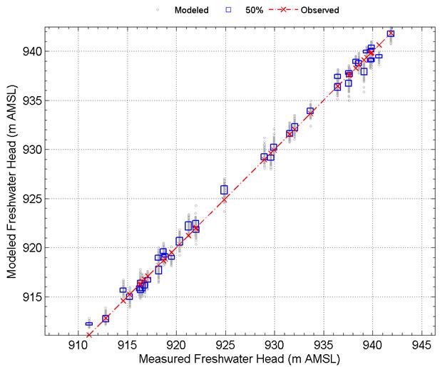
Figure TFIELD 5-24. Results for 42 Total Steady-state Head Measurements for the 100 Selected Fields (No SNL-6 or SNL-15). Observed heads are red ×'s along the diagonal line.
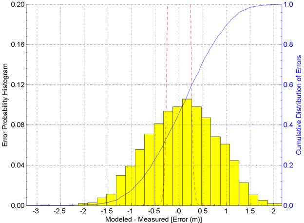
Figure TFIELD 5-25. Histogram of Steady-state Head Errors for the 100 Selected Fields (No SNL-6 or SNL-15). Red dashed line is the ±3σ
section of the measurement error PDF. The slight skew to right is an artifact of the binning.
The work described in Section TFIELD-6.0 was completed under AP-144, Analysis Plan for the Calculation of Culebra Flow and Transport for CRA-2009 PABC (Kuhlman 2009). The modifications used for CRA-2009 PABC still apply to CRA 2014, and are therefore discussed here.
PA models two categories of mining-impacted transmissivity fields: partial mining with only mining outside the LWB, and full mining with regions both inside and outside the LWB mined.
The CRA-2009 PABC Culebra T-field mining modifications basically follow the procedure used in CRA-2004 PABC (Lowry and Kanney 2005), with two exceptions: 1) a new definition of the region containing minable potash is used, and 2) the new T-fields in Sections TFIELD-3.0 through TFIELD-5.0 are used as inputs. The procedure for the mining modification portion of the analysis is summarized below:
1. Obtain the sampled values for the random mining modification factor (100 vectors × 3 replicates);
2. Map potential areas of future potash mining onto the groundwater modeling domain for both full- and partial-mining scenarios;
3. Apply the mining modification factor to the 100 stochastically calibrated T-fields from AP-114 Task 7 (Hart et al. 2009), producing 600 mining-modified T-fields (100 vectors × 2 mining scenarios × 3 replicates);
4. Perform steady-state flow simulations for each of the 600 mining-modified T-fields using MODFLOW-2000; and
5. Perform particle tracking using the new mining-affected flow-fields to determine advective travel times to the WIPP LWB.
Potash mining in the region surrounding the WIPP involves underground excavation in the McNutt Potash zone of the upper Salado Formation, which is located stratigraphically above the WIPP repository horizon but below the Culebra Member of the Rustler Formation (see Figure TFIELD 2-1). It is hypothesized that subsidence due to collapse of the underground voids created in the McNutt potash zone during mining will lead to increased permeability in the Rustler Formation, due to increased fracturing, similar to the Salado dissolution zone effects in Figure TFIELD 2-2. The purpose of the mining scenario calculations is to determine the impact of potash mining on groundwater flow directions and transport velocities in the Culebra. This analysis largely represents a re-application of the methods used in CRA-2004 PABC (Lowry and Kanney 2005), with a few minor exceptions:
1. The definition of the regions where minable potash is believed to exist has been updated, as obtained from the Bureau of Land Management (BLM) (Cranston 2009).
2. The configuration of the MODFLOW model that mining modifications are being applied to has changed (see Sections TFIELD-3.0 through TFIELD-5.0).
3. The way the mining-modified areas interact with specified head areas of the flow model has changed, due to the change in the boundary conditions (there were no specified head areas inside the CRA-2004 PABC MODFLOW model).
This section describes the CRA-2009 PABC effort in characterizing mining effects in the Culebra and highlights the differences and additions relative to past calculations (Ramsey and Wallace 1996; Lowry 2003a, Lowry 2003b, and Lowry 2004). The reader is encouraged to review the past documents for further background information. There have been no changes to the mining modifications procedure or data for CRA-2014 since CRA-2009 PABC.
Starting with the 100 calibrated T-fields from Section TFIELD-5.0, T-fields are modified to reflect the effects of mining by multiplying the transmissivity value in cells that lie within designated mining zones by a random factor uniformly sampled between 1 and 1000. The range of this factor is set by the U.S. Environmental Protection Agency (EPA) in regulation 40 CFR 194.32(b) (U.S. EPA 1996). The scaling factor for each T-field is provided by Latin hypercube sampling (Kirchner 2010).
A forward steady-state flow simulation is run for each new T-field under each mining scenario (full and partial) across three replicates of mining factors, resulting in 600 simulations. Particle tracking is performed on both the 100 original and 600 modified flow-fields to compare the flow path and groundwater travel time from a point above the center of the WIPP disposal panels to the LWB. Cumulative distribution functions (CDFs) are produced for each mining scenario and compared to the undisturbed scenario. The CDFs indicate the probability a conservative tracer (i.e., a marked water particle) would reach the WIPP LWB during a given interval of time, flowing in the Culebra under a natural gradient. In addition to comparing travel times, particle-tracking directions are also examined to determine the effect on the regional flow direction in the WIPP area due to mining.
The eastern limit of the MODFLOW model domain used in the CRA-2009 PABC analysis (Hart et al. 2008) was extended eastward, compared to the MODFLOW domain used in the CRA-2004 PABC analysis. This change was made to locate the boundary in an area where halite is present in all of the non-dolomite members of the Rustler Formation, simplifying the specification of the eastern model boundary condition. See Section TFIELD-3.1 for CRA-2009 PABC MODFLOW model construction details.
Like the model domain and discretization, the boundary and initial conditions used in CRA-2009 PABC are described fully in AP-114 Task 7 (Hart et al. 2009). Regional flow rates within the flow model are controlled by the boundary conditions and the hydraulic conductivity distribution. The regional gradient across the domain was approximately
(943.9 m - 911.6 m)/30.7 km = 0.00105 (TFIELD 6.1)
The gradient across the model domain was computed by averaging the constant heads along the northernmost portion of the northern boundary (row 1, columns 1-140, 943.9 m), subtracting the average heads along the entire southern boundary (911.6 m), and dividing by the north-south model domain extent (30.7 km). It was assumed that mining impacts would not significantly change this regional gradient and thus the specified initial conditions for the mining scenarios are identical to those in AP-114 Task 7 (Hart et al. 2009). In addition, the CCA, CRA-2004, and CRA-2004 PABC all used this same conceptualization (keeping the outer boundary conditions fixed between the mining and non-mining scenarios). The same conceptualization was maintained in the CRA-2009 PABC model to facilitate comparisons between the different models.
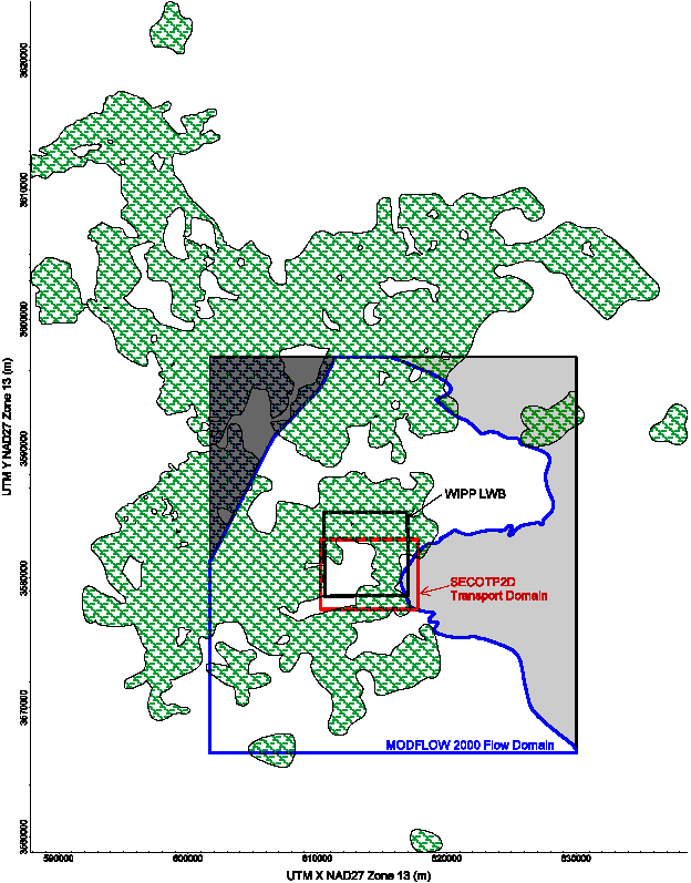
Figure TFIELD 6-1. Comparison of Minable Potash Area to the Flow and Transport Modeling Domains. Green hatches represent minable potash area (Cranston 2009).
The 2009 version of the BLM map delineating distribution of minable potash ore was obtained from BLM as an ESRI shapefile (Cranston 2009), plotted in Figure TFIELD 6-1. The process to convert this shapefile to a grid of integers corresponding to Culebra MODFLOW model cells (indicating whether a model cell was affected by mining or not) is explained in Appendix 1 of Kuhlman (Kuhlman 2010).
Since the potash-mining horizon is located in the Salado Formation below the Culebra, the areas disturbed by mining activities in the Culebra are larger than mined areas in the Salado due to angle-of-draw effects. Subsidence effects will not propagate up vertically, but instead will propagate up and out at 45° angles between horizontal and vertical. Based on an average distance from the McNutt potash zone to the Culebra, a 253-m-wide collar was added to the mining-impacted areas (consistent with that done previously; see Ramsey and Wallace (Ramsey and Wallace 1996) and Bertram (Bertram 1995). This was considered a conservative estimate of the angle-of-draw effects. To accommodate the angle of draw, the mining zone boundaries, as overlaid on the current model grid, were extended outward three cells (300 m) in the x- and y-directions, and two cells (283 m) in the diagonal directions (see Figure TFIELD 6-2 for an illustration of the mining-expansion stencil).
|
|
|
|
A
|
|
|
|
|
|
A
|
A
|
A
|
A
|
A
|
|
|
|
A
|
A
|
A
|
A
|
A
|
|
|
A
|
A
|
A
|
M
|
A
|
A
|
A
|
|
|
A
|
A
|
A
|
A
|
A
|
|
|
|
A
|
A
|
A
|
A
|
A
|
|
|
|
|
|
A
|
|
|
|
Figure TFIELD 6-2. Stencil Used to Model Cells Affected by Mining-related Subsidence (Blue Cells with A) Due to Mining in Red "M" Cell, Using 45° Angle of Draw
Figure TFIELD 6-3 shows the CRA-2009 PABC modeling domain and mining zones for the full-mining case in comparison to the 1996 CCA and the CRA-2004 delineations. The comparison of the current and previous partial-mining cases is shown in Figure TFIELD 6-4. A close-up of the WIPP site and the distribution of minable potash is shown in Figure TFIELD 6-5, which illustrates how the definition inside the WIPP LWB has changed significantly since CRA-2004 PABC. For CRA-2004 PABC, the closest minable potash was approximately 1,230 m from the center of the WIPP panels in the southeast direction; for CRA-2009 PABC, this distance was reduced to approximately 670 m (in a more easterly direction).
The output of this mining-area delineation was a mining effects indicator field. A value of 1 means the model cell lies within a potential mining-affected zone, and a value of 0 means that it is outside a potential mining-affected zone.
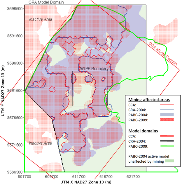
Figure TFIELD 6-3. Definitions of Mining-affected Areas in Full-mining Scenario Between Current and Previous Models. Base image is Figure 3.2 from Lowry and Kanney (2005). CRA-2009 PABC mining area (red stippled area) and model domain (green line) definitions are current definitions used in CRA-2014.
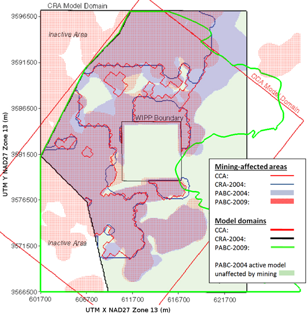
Figure TFIELD 6-4. Definitions of Partial-mining-affected Areas Between Current and Previous Applications. Base image is Figure 3.3 from Lowry and Kanney (2005). CRA-2009 PABC mining area (red stippled area) and model domain (green line) definitions are current definitions used in CRA-2014.
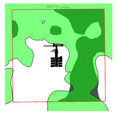
Figure TFIELD 6-5. Comparison of Minable Potash Distribution Inside the WIPP LWB for CRA-2004 PABC (Dark Gray) and CRA-2009 PABC (Translucent Green). The WIPP repository plan is shown for comparison, from Figure 3.6 of Lowry and Kanney (2005).
The calibration process in Section TFIELD-5.0 produced 100 sets of T, A, S, and R fields that each minimize the error between observed and model-calculated head distributions. To simulate the effects of mining, the field of T values from each realization was multiplied by its own unique mining scaling factor in areas of potential mining, and MODFLOW was re-run with these mining-modified T-fields to produce the mining-affected head and flow distributions. The other parameter fields (S, A, and R) were not modified in the process. The cell-by-cell flow budget files were used in particle tracking and radionuclide transport calculations. Three different sets of mining factors were used, each set forming a replicate (given here as R1, R2, and R3). Thus, for each mining scenario (full and partial), three sets of 100 mining-altered T-fields and related cell-by-cell flow budgets were produced.
In each realization, a single conservative particle was tracked from the UTM NAD27 coordinate
x = 6,135,975 m, y = 35,813,852 m (i.e., the Culebra location of monitoring well C-2737, directly above the center of the WIPP waste panels) to the LWB for each combination of T-field, replicate, and mining scenario using the SNL-developed particle-tracking code DTRKMF. Two main outputs were generated from the suite of particle tracks. First, plots were constructed showing the individual tracks for all 100 T-fields in each scenario for each replicate (six plots total). This allows visual comparison of the prevailing flow directions for the full- and partial-mining scenarios and the qualitative comparison of the variability of the tracking direction. Secondly, CDFs were constructed for each replicate and scenario, which describe the probability that a water particle will cross the LWB in a given amount of time. The six plots and the CDFs are presented in Section TFIELD-6.3.
Particle tracks were computed using DTRKMF (Rudeen 2003), which uses the binary cell-by-cell flow budget files produced by MODFLOW-2000. In flow calculations, the full 7.75 m thickness of the Culebra is used, while for transport and particle-tracking purposes the thickness is reduced to 4.0 m to focus all flow through the lower, more permeable portion of the Culebra (Holt 1997). A value of 16% porosity was used for the particle-tracking calculations (parameter DPOROS). Porosity directly affects transport, but is not needed for the calibration of the flow model.
Particle tracking was performed to allow plotting and quantitative comparison between the two mining scenarios and the non-mining scenario, which was not used in the PA SECOTP2D radionuclide transport calculations. The particle-tracking results illustrate the advective pathway taken by a marked water particle. They do not take into consideration retardation, dispersion, or molecular diffusion, which may be accounted for in PA by radionuclide transport. The particle tracks also allow easier comparison of the 600 results (each a 1D trace) in a single plot, in contrast to showing 600 plots of concentrations (each a 2D field) produced from SECOTP2D.
Compared to the non-mining scenario (results already given in AP-114 Task 7 (Hart et al. 2009)), the travel times for the partial-mining scenarios are longer, while travel times for the full-mining scenarios are shorter. The median travel time across all three replicates for the full-mining scenario is approximately 0.689 times the median travel time of the non-mined scenario (see Table TFIELD 6-1, Figure TFIELD 6-6, and Figure TFIELD 6-7 for summary statistics and comparison to CRA-2004 PABC results). All advective particle travel times are plotted, but it should be noted that the regulatory limit for radionuclide transport modeling is 10,000 years, taking into consideration retardation, diffusion, and dispersion (which do not apply to particle track modeling). The median travel time across all three replicates for the partial-mining scenario is 3.034 times greater than for the non-mining scenario. For CRA-2004 PABC, travel times in both the full- and partial-mining scenarios were slower (longer) than for the non-mining scenario. The CDFs for the full-, partial-, and non-mining scenarios are shown in Figure TFIELD 6-6. Travel times from CRA-2009 PABC for particles in the non-mining scenario are closer to CCA travel times than those from CRA-2004 PABC (Figure TFIELD 6-7).
Table TFIELD 6-1. Particle-tracking Travel-time Statistics from Center of the WIPP Panels to the WIPP LWB (Years). Global statistics for full and partial mining include 300 realizations, while no mining only includes 100 realizations.
|
|
CRA-2009 PABC
|
CRA-2004 PABC
|
|
Replicate
|
Statistic
|
Full
|
Partial
|
No Mining
|
Full
|
Partial
|
No Mining
|
|
R1
|
Median
|
5,138
|
22,581
|
N/A
|
64,026
|
117,815
|
N/A
|
|
Max
|
200,260
|
91,119
|
2,175,165
|
2,727,191
|
|
Min
|
1,591
|
5,042
|
2,130
|
5,185
|
|
R2
|
Median
|
4,956
|
21,999
|
80,801
|
148,489
|
|
Max
|
94,852
|
84,929
|
2,059,263
|
1,667,084
|
|
Min
|
1,421
|
5,037
|
2,463
|
4,855
|
|
R3
|
Median
|
5,560
|
22,537
|
74,315
|
118,919
|
|
Max
|
93,172
|
86,758
|
1,779,512
|
3,128,693
|
|
Min
|
1,421
|
4,505
|
2,507
|
3,314
|
|
Global
|
Median
|
5,084
|
22,376
|
7,374
|
70,170
|
131,705
|
18,289
|
|
Max
|
200,260
|
91,119
|
73,912
|
2,175,165
|
3,128,693
|
101,205
|
|
Min
|
1,421
|
4,505
|
2,618
|
2,130
|
3,314
|
3,111
|
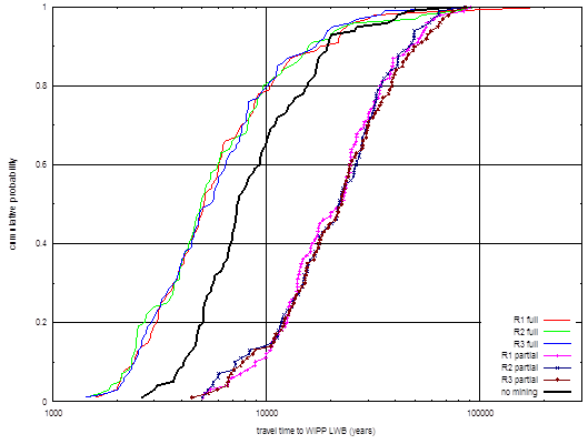
Figure TFIELD 6-6. CDF of Advective Particle Travel Times From the Center of the WIPP Waste Panels To the WIPP LWB for Full, Partial, and Non-mining Scenarios
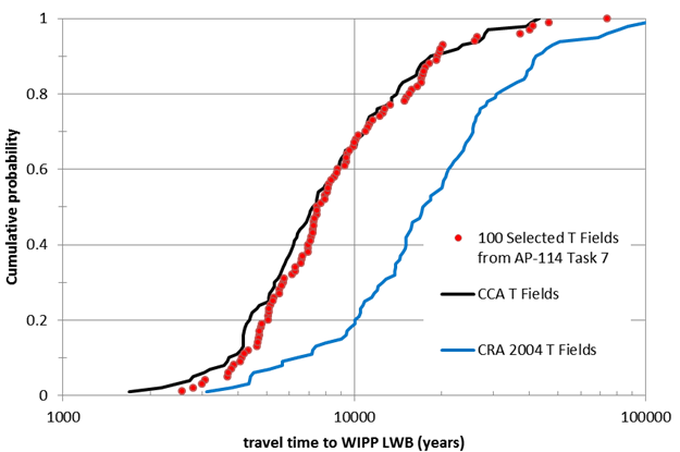
Figure TFIELD 6-7. Comparison of Advective Particle Travel Time CDFs for Non-mining Scenarios of CRA-2009 PABC, CRA-2004 PABC, and CCA. Travel times are from the center of the WIPP waste panels to the WIPP LWB.
The particle track directions for the non-, full-, and partial-mining scenarios for CRA-2009 PABC are illustrated in Figure TFIELD 6-8 to Figure TFIELD 6-11. Figure TFIELD 6-13 shows the non-mining case particle tracks all the way to the edge of the MODFLOW model domain, rather than only to the WIPP LWB. Like past mining scenario calculations (i.e., CRA-2004 PABC), there is a strong similarity between the three replicates (R1, R2, and R3) for each scenario (full or partial mining), although the travel directions for the CRA-2009 PABC are different than for the CRA-2004 PABC (Lowry and Kanney 2005). A larger amount of minable ore exists inside the WIPP LWB, especially the ore immediately to the east of the particle release point. This leads to different effects of full mining on travel times compared to CRA-2004 PABC.
The high-T pathway in the southeastern portion of the WIPP site (Figure TFIELD 5-15) was more accurately represented in CRA-2009 PABC results, compared to CRA-2004 PABC results. This difference in the underlying flow field calibration is another source of difference between CRA-2004 PABC and CRA-2009 PABC particle-tracking results.
In CRA-2009 PABC, nearly all particles immediately go east to this boundary and then move south along it towards to the edge of the LWB at approximately x = 612.75 km (see Figure TFIELD 6-9 and Figure TFIELD 6-12). This is in contrast to the partial-mining scenario where the tracking directions are more similar to the non-mining scenario, but more evenly distributed spatially along the southern boundary. In the non-mining scenario, most of the particles exit near the high-transmissivity zone at approximately x = 615 km.
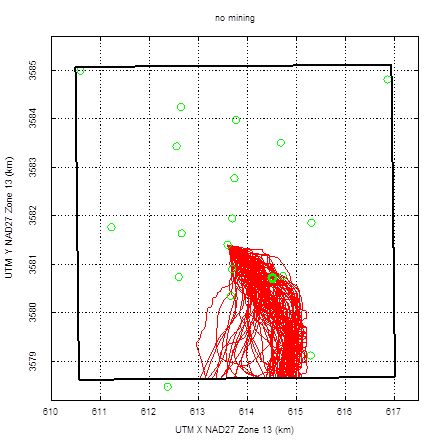
Figure TFIELD 6-8. 100 Particle Tracks for Non-mining Scenario. Black box is the WIPP LWB, green circles are Culebra monitoring well locations.
Figure TFIELD 6-9. 100 Particle Tracks Each for R1 Full and Partial Mining Scenarios. Small magenta squares and blue crosses indicate centers of MODFLOW cells located within potash and mining-affected areas, respectively; thin black line is minable potash.
Figure TFIELD 6-10. 100 Particle Tracks Each for R2 Full- and Partial-mining Scenarios. Small magenta squares and blue crosses indicate centers of MODFLOW cells located within potash and mining-affected areas, respectively; thin black line is minable potash.
Figure TFIELD 6-11. 100 Particle Tracks Each for R3 Full- and Partial-mining Scenarios. Small magenta squares and blue crosses indicate centers of MODFLOW cells located within potash and mining-affected areas, respectively; thin black line is minable potash.
High-T areas corresponding to the mining-affected zones create preferential pathways through the system (e.g., see oranges and yellows in Figure TFIELD 6-14). These preferential pathways result in higher velocities and flow rates through the mining zone and therefore relatively slower velocities in the non-mined areas. In the partial-mining scenario, where there is no mining inside the WIPP LWB, the preferential pathway goes "around" the LWB, rather than through it (similar to behavior seen in both mining scenarios for CRA-2004 PABC). In the full-mining scenario, the potentially mined regions are closer to the release point than in CRA-2004 PABC (see Figure TFIELD 6-5 for comparison), giving the particles a high-T pathway from the release point to the LWB, resulting in shorter travel times than the non-mined scenario. This behavior is different from that predicted with the CRA-2004 PABC model. A comparison of the median, maximum, and minimum travel times for each scenario is presented in Table TFIELD 6-1.
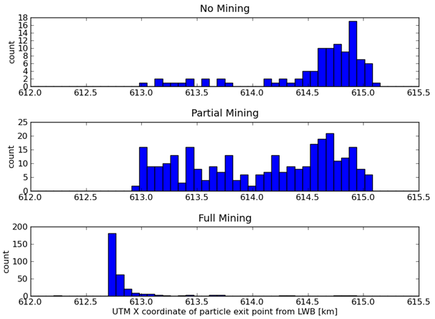
Figure TFIELD 6-12. Histograms of Particle x-coordinates at Exit Point From LWB. Full- and partial-mining include all three replicates (note different vertical scales between plots; no mining contains 100 particles while mining scenarios each include 300 particles).
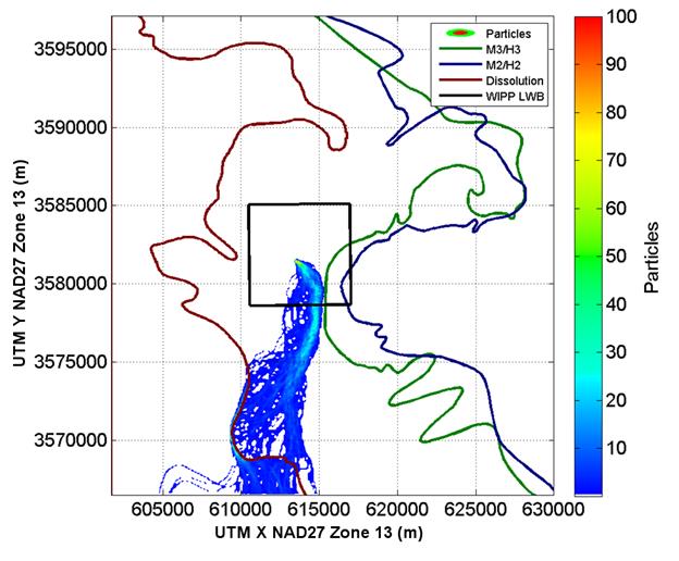
Figure TFIELD 6-13. Particle Counts in Each Cell Across All 100 Selected Realizations for Non-mining Scenario
Figure TFIELD 6-14. Magnitude of Darcy Flux for a Single Realization (r440) for No, Partial, and Full-mining Scenarios Using Cell-based Coordinates. LWB (black) and SECOTP2D transport model domains (red) shown for reference.
Instantaneous speeds (the magnitude of particle velocities) were calculated from the DTRKMF particle locations and times using backwards finite differences,
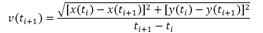 (TFIELD 6.2)
where a subscript i indicates the previous time step (a record or line in the DTRKMF output file) and a subscript i+1 is the current time step. This approach assumes a straight line connects the locations at the beginning and ends of the step, so it is potentially underestimating speeds, but step sizes are small and error should be minimal. These values should be used for qualitative comparisons between realizations and scenarios, rather than quantitative estimates of true particle velocities.
In Figure TFIELD 6-15 through Figure TFIELD 6-18, the color of the diamond indicates the particle velocity; the dots are located at the midpoint of the step, e.g.,
x
midpt = ½[x(ti
) + x(ti
+1)], y
midpt = ½[y(ti
) + y(ti
+1)]. In the no-mining case (Figure TFIELD 6-15), the highest particle velocities are in the southeastern portion of the particle swarm, corresponding to the high-transmissivity pathway (Hart et al. 2009) exiting the LWB at approximately
x = 614,750 m (Figure TFIELD 6-12). This high-T pathway has been observed in multi-well pumping tests, and was intentionally included in the soft data used to create the base T-fields (Section TFIELD-4.2.3). This high-T pathway was not as prevalent in the CRA-2004 PABC model calibration results.
The effects of the full-mining scenario are clearly evident in the left halves of Figure TFIELD 6-16 through Figure TFIELD 6-18. High particle velocities (yellows and oranges) are found along the margin of the mining-affected areas, where particles enter the increased-T region. For comparison, in the partial-mining scenario the particles are relatively slowed down and more evenly distributed in the region between the release point and the southern WIPP LWB, with the only high velocities found in the high-T pathway in the southeast, similar to the no-mining scenario (Figure TFIELD 6-15).
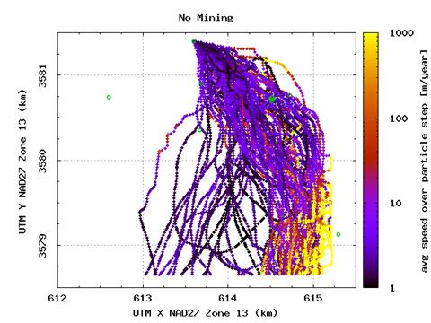
Figure TFIELD 6-15. Particle Speeds for Non-mining Scenario Computed from DTRKMF Results. Open symbols are Culebra well locations.
Figure TFIELD 6-16. Particle Speeds for R1, Computed From DTRKMF Results. Open symbols are Culebra well locations.
Figure TFIELD 6-17. Particle Speeds for R2, Computed From DTRKMF Results. Open symbols are Culebra well locations.
Figure TFIELD 6-18. Particle Speeds for R3, Computed from DTRKMF Results. Open symbols are Culebra well locations.
Correlation analysis for the CRA-2009 PABC particle-tracking calculations shows that travel time and the random mining factor have weak positive correlation with the full-mining (Figure TFIELD 6-19) or partial-mining (Figure TFIELD 6-20) scenarios. Larger mining factors are weakly correlated with longer travel times. This is similar to what was observed for CRA-2004 PABC (Lowry and Kanney 2005). The high scatter in Figure TFIELD 6-19 and Figure TFIELD 6-20 indicates that the transmissivity spatial distribution plays the more significant role in determining the travel time than the mining factor does. See Appendix 1 of Kuhlman (Kuhlman 2010) for a cross-sectional comparison of transmissivity for each mining type, showing that the variability in the transmissivity due to calibration is on the same order as that due to mining for a single realization. The mining factor plays a weak but slightly larger role in explaining the observed variance for the partial-mining realizations (Figure TFIELD 6-20) than the full-mining realizations (Figure TFIELD 6-19), based on the larger (but still relatively small) R2 value for the straight-line fit of log10 travel times to mining factors.
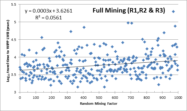
Figure TFIELD 6-19. Correlation of Mining Factor and Travel Time to the WIPP LWB for Full-mining Scenario (All Replicates)
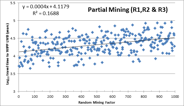
Figure TFIELD 6-20. Correlation of Mining Factor and Travel Time to the WIPP LWB for Partial-mining Scenario (All Replicates)
The 100 transmissivity fields resulting from calibration to both steady-state and transient observed freshwater heads in the Culebra (Section TFIELD-5.1) were modified to account for potential effects due to mining potash from the Salado Formation above the repository. A definition of the areal extent of minable potash was obtained from the BLM (Cranston 2009) and used to define areas where Culebra transmissivity was increased by a randomly sampled mining factor (1 ≤ MINP_FACT ≤ 1000). Two mining scenarios were developed: a full-mining scenario with all minable potash removed and a partial-mining scenario with only potash outside the WIPP LWB removed.
The mining-modified transmissivities were inputs to a MODFLOW flow model, which produced budget files used by DTRKMF to compute advective particle tracks from a release point at the center of the WIPP waste panels (C-2737) to the edge of the WIPP LWB. Results show that for the partial-mining scenario, the median particle travel time of 22,376 years is 3.03 times greater than for the non-mining scenario (7,374 years); the median particle travel time for the partial-mining scenario in CRA-2004 PABC was 7.06 times greater than for the non-mining scenario. In contrast to the CRA-2004 PABC, the full-mining scenario decreased median travel time to 5,084 years, a factor of 1.45 faster than for the non-mining scenario; the median particle travel time for the full-mining scenario in CRA-2004 PABC was 3.84 times slower than for the non-mining scenario. For the partial-mining scenario, the increase in transmissivity due to mining increases the relative flow rate through the mining zones, with a corresponding decrease in flow through the non-mining zones. This decrease in flow through the non-mining zones produces longer travel times for the partial-mining scenario. For the full-mining scenario, the potash definition from BLM (Cranston 2009) locates minable potash ore much closer to the C-2737 release point than in CRA-2004 PABC (see Figure TFIELD 6-5). This new shortened distance from the release point to the nearest minable potash (in the full-mining scenario) reverses the slowing-down trend observed in the CRA-2004 PABC analysis.
As in the CRA-2004 PABC calculations, a very weak positive correlation was found between the travel times and the random mining factor (the higher the random mining factor, the longer the particle travel time - see Figure TFIELD 6-19 and Figure TFIELD 6-20). As the mining factor is increased, the flow through the non-mining areas (including the C-2737 particle release location) is decreased, producing longer travel times and the positive correlation. Most of the advective particle travel time variability is due to differences in the base T-fields and their subsequent calibration, and not the random mining factor.
Observed Culebra transmissivities (T) have been related to four deterministic factors: the thickness of overburden above the Culebra, the presence or absence of dissolution of the upper Salado, the presence of gypsum cements, and the presence or absence of halite in units above and below the Culebra. Culebra T is also related to the occurrence of open, interconnected fractures that cannot be mapped as easily as the other three factors and therefore must be treated stochastically. A linear-regression model for Culebra T has been developed based on these factors that provided an excellent match to the observed data, and can be tested through the collection of additional data. This model was used to create 1000 stochastic realizations of the distribution of Culebra T (base T-fields) in the vicinity of the WIPP site.
A MODFLOW-2000 modeling domain was defined extending 30.7 km north-south and 28.4 km east-west, roughly centered on the WIPP site. This domain was discretized into 87,188 uniform 100-m square two-dimensional finite-difference cells. An inactive portion of the northwest corner of the domain is used to represent a no-flow boundary along the axis of Nash Draw. A low-permeability constant-head portion of the eastern section of the domain is used to represent the lithostatic pressure portion of the Culebra sandwiched above and below by Rustler halite units. Freshwater head observations in 42 monitoring wells from May 2007 were used as steady-state calibration targets. Drawdown observations in 62 observation wells, in response to 9 unique pumping tests, were used as transient calibration targets. A subset consisting of 100 of the 200 calibrated Culebra model realizations were selected based on their ability to simulate these observed heads.
The EPA requires that the potential effects of future potash mining be taken into account when evaluating the performance of the WIPP disposal system. Accordingly, T in the areas within the model domain where current or future mining might affect the Culebra were scaled by a random multiplier between 1 and 1,000 obtained from Latin hypercube sampling. A single multiplier was used for each T-field, applied first to the areas outside the WIPP LWB that might be mined to create a partial-mining T-field, and then to all areas (both inside and outside the WIPP LWB) to create a full-mining T-field. Three statistically similar replicates of mining multipliers were generated, leading to a total of 600 unique T-fields (100 calibrated realizations, 2 mining scenarios, and 3 replicates). The MODFLOW-2000 flow budgets were used from each realization as input for both advective particle tracking (DTRKMF) summarized here and radionuclide solute transport (SECOTP2D) used in WIPP PA.
The non-mined travel times from the center of the WIPP waste panels to the WIPP LWB are similar to those computed for the CCA and therefore faster than those computed for CRA-2004 PABC. The decrease in travel time to the LWB can be attributed to the presence of a consistent high-transmissivity pathway leaving the south-east portion of the LWB. The presence of this pathway is supported by observed drawdown data from the SNL-14 pumping test.
In the partial-mining case, particle tracks show increased travel times from the center of the WIPP waste panels to the WIPP LWB, compared to the non-mining scenario. In the full-mining case, particle tracks showed decreased travel times to the WIPP LWB, due to the close proximity of minable potash to the center of the WIPP waste panels.
(*Indicates a reference that has not been previously submitted.)
Beauheim, R.L. 1987a. Analysis of Pumping Tests of the Culebra Dolomite Conducted at the H-3 Hydropad at the Waste Isolation Pilot Plant (WIPP) Site. Albuquerque, NM: Sandia National Laboratories. SAND86-2311. [PDF / Author]
Beauheim, R.L. 1987b. Interpretation of the WIPP-13 Multipad Pumping Test of the Culebra Dolomite at the Waste Isolation Pilot Plant (WIPP) Site. Albuquerque, NM: Sandia National Laboratories. SAND87-2456. [PDF / Author]
Beauheim, R.L. 1989. Interpretation of H-11b4 Hydraulic Tests and the H-11 Multipad Pumping Test of the Culebra Dolomite at the Waste Isolation Pilot Plant (WIPP) Site. Albuquerque, NM: Sandia National Laboratories. SAND89-0536. [PDF / Author]
Beauheim, R.L. 2007. Diffusivity mapping of fracture interconnections. In Proceedings of the 2007 US EPA/NGWA Fractured Rock Conference. Westerville, OH, 2007. National Ground Water Association. [Author]
Beauheim, R.L. 2008. Analysis Plan for Evaluation and Recalibration of Culebra Transmissivity Fields AP-114, Revision 1. Carlsbad, NM: Sandia National Laboratories. [PDF / Author]
Beauheim, R.L. 2009. Changes to Culebra T-Field Calibration Procedures under AP-114 Task 7. Carlsbad, NM: Sandia National Laboratories. ERMS 551437. [PDF / Author]
Beauheim, R.L. and R.M. Holt. 1990. Geological and Hydrological Studies of Evaporites in the Northern Delaware Bains for the Waste Isolation Pilot Plant (WIPP). In D.W. Powers, R.M. Holt, R.L. Beauheim and N. Rempe, eds. Guidebook 14. Geological Society of America (Dallas Geological Society). pp.45-78. [Author]
Beauheim, R.L. and G.J. Ruskauff. 1998. Analysis of Hydraulic Tests of the Culebra and Magenta Dolomites and Dewey Lake Redbeds Conducted at the Waste Isolation Pilot Plant Site. Albuquerque, NM: Sandia National Laboratories. SAND98-0049. [PDF / Author]
Bertram, S.G. 1995. Record of FEP Screening Work, FEP ID#NS-11: Subsidence Associated with Mining Inside or Outside the Controlled Area. Carlsbad, NM: Sandia National Laboratories. ERMS 230761. [PDF / Author]
Bowman, D.O. and R.M. Roberts. 2008. Analysis Report for AP-070, Analysis of Hydraulic Tests Performed in IMC-461, SNL-6, H-11b2, H-15, and C-2737. Carlsbad, NM: Sandia National Laboratories. ERMS 539221. [Author]
Burgess, A., T. Doe, T. Lowenstein, and J.A. Thies. 2008. Waste Isolation Pilot Plant Culebra Hydrogeologicy Conceptual Model Peer Review Final Report. Carlsbad, NM: U.S. Department of Energy. ERMS 551513. [PDF / Author]
Chavez, M. 2006. NP 19-1 Software Requirements, Revision 12. Carlsbad, NM: Sandia National Laboratories. [PDF / Author]
Clayton, D.J., R.C. Camphouse, J.W. Garner, A.E. Ismail, T.B. Kirchner, K.L. Kuhlman, and M.B. Nemer. 2010. Summary Report of the CRA-2009 Performance Assessment Baseline Calculation. Carlsbad, NM: Sandia National Laboratories. ERMS 553039. [PDF / Author]
Cranston, C.C. 2009. Minable Potash Ore. Carlsbad, NM: Bureau of Land Management. ERMS 551120. [PDF / Author]
Currie, J.B. and S.O. Nwachukwu. 1974. Evidence on incipient fracture porosity in reservoir rocks at depth. Bulletin of Canadian Petroleum Geology. 22, pp.42-58. [Author]
Deutsch, C.V. and A.G. Journel. 1998. GSLIB: Geostatistical Software Library and User's Guide. 2nd ed. New York: Oxford University Press. [Author]
Doherty, J. 2000. PEST Manual. Brisbane, Australia: Watermark Numerical Computing. [Author]
Harbaugh, A.W., E.R. Banta, M.C. Hill, and M.G. McDonald 2000. MODFLOW 2000: The U.S. Geological Survey Modular Ground-Water Model User Guide. Reston, VA: U.S. Geological Survey. OFR 00-92. [PDF / Author]
Hart, D.B., R.L. Beauheim, and S.A. McKenna. 2009. Analysis Report for Task 7 of AP-114: Calibration of Culebra Transmissivity Fields. Carlsbad, NM: Sandia National Laboratories. ERMS 552391. [PDF / Author]
Hart, D.B., R.M. Holt, and S.A. McKenna. 2008. Analysis Report for Task 5 of AP-114: Generation of Revised Base Transmissivity Fields. Carlsbad, NM: Sandia National Laboratories. ERMS 549597. [PDF / Author]
Holt, R.M. 1997. Conceptual Model for Transport Processes in the Culebra Dolomite Member of the Rustler Formation. Albuquerque, NM: Sandia National Laboratories. SAND97-0194. [PDF / Author]
Holt, R.M., R.L. Beauheim, and D.W. Powers. 2005. Predicting fractured zones in the Culebra Dolomite. In B. Faybishenko, P.A. Witherspoon and J. Gale, eds. Dynamics of Fluids and Transport in Fractured Rock. American Geophysical Union. pp.103-16. [Author]
Holt, R.M. and D.W. Powers. 1988. Facies variability and post-depositional alteration within the Rustler Formation in the vicinity of the Waste Isolation Pilot Plant, southeastern New Mexico. Carlsbad, NM: Department of Energy. WIPP-DOE-88-004. [PDF / Author]
Holt, R.M. and L. Yarbrough. 2002. Analysis Report, Task 2 of AP-088, Estimating Base Transmissivity Fields. Carlsbad, NM: Sandia National Laboratories. ERMS 523889. [PDF / Author]
Johnson, P.B. 2009a. Potentiometric Surface, Adjusted to Equivalent Freshwater Heads, of the Culebra Dolomite Member of the Rustler Formation near the WIPP Site, Revision 1. Carlsbad, NM: Sandia National Laboratories. ERMS 548746. [PDF / Author]
Johnson, P.B. 2009b. Routine Calculations Report In Support of Task 6 of AP-114: Potentiometric Surface, Adjusted to Equivalent Freshwater Heads, of the Culebra Dolomite member of the Rustler Formation near the WIPP Site, Revision 2. Carlsbad, NM: Sandia National Laboratories. ERMS 551116. [PDF / Author]
Kirchner, T.B. 2010. Generation of the LHS Samples for the AP-145 (PABC09) PA Calculations. Carlsbad, NM: Sandia National Laboratories. ERMS 552905. [PDF / Author]
Kuhlman, K.L. 2009. AP-144 Analysis Plan for the Calculation of Culebra Flow and Transport for CRA2009PABC. Carlsbad, NM: Sandia National Laboratories. ERMS 551676. [PDF / Author]
Kuhlman, K.L. 2010. Analysis Report for the CRA-2009 PABC Culebra Flow and Transport Calculations (AP-144). Carlsbad, NM: Sandia National Laboratories. ERMS 552951. [PDF / Author]
Leigh, C.D., J.F. Kanney, L.H. Brush, J.W. Garner, G.R. Kirkes, T. Lowry, M.B. Nemer, J.S. Stein, E.D. Vugrin, S. Wagner, and T.B. Kirchner. 2004. 2004 Compliance Recertification Application Performance Assessment Baseline Calculation, Revision 0. Carlsbad, NM: Sandia National Laboratories. ERMS 541521. [PDF / Author]
Lowry, T.L. 2003a. Analysis Report, Task 5 of AP-088: Evaluation of Mining Scenarios. Carlsbad, NM: Sandia National Laboratories. ERMS 531138. [PDF / Author]
Lowry, T.L. 2003b. Analysis Report, Tasks 2 & 3 of AP-100: Grid Size Conversion and Generation of SECOTP2D Input. Carlsbad, NM: Sandia National Laboratories. ERMS 531137. [PDF / Author]
Lowry, T.S. 2004. Analysis Report for Inclusion of Omitted Areas in Mining Transmissivity Calculations in Response to EPA Comment G-11. Carlsbad, NM: Sandia National Laboratories. ERMS 538218. [PDF / Author]
Lowry, T.S. and J.F. Kanney. 2005. Analysis Report for the CRA-2004 PABC Culebra Flow and Transport Calculations. Carlsbad, NM: Sandia National Laboratories. ERMS 541508. [PDF / Author]
McKenna, S.A. and D.B. Hart. 2003. Analysis report for Task 4 of AP-088: Conditioning of Base T Fields to Transient Heads. Carlsbad, NM: Sandia National Laboratories. ERMS 531124. [PDF / Author]
McKenna, S.A. and A. Wahi. 2006. Local Hydraulic Gradient Estimator Analysis of Long-Term Monitoring Networks. Ground Water. 44(5), pp.723-31. [Author]
Mehl, S.W. 2001. MODFLOW-2000, The US Geological Survey Modular Ground-Water Model User Guide to the Link-AMG (LMG) Package for Solving Matrix Equations using an Algebraic Multigrid Solver. USGS (US Geological Survey). OFR 01-177. [PDF / Author]
Powers, D.W. 2002a. Analysis report Task 1 of AP-088, Construction of geologic contour maps. Carlsbad, NM: Sandia National Laboratories. ERMS 522085. [PDF / Author]
Powers, D.W. 2002b. Addendum to Analysis Report, Task 1 of AP-088, Construction of Geologic Contour Maps. Carlsbad, NM: Sandia National Laboratories. ERMS 523886. [PDF / Author]
Powers, D.W. 2003. Addendum 2 to Analysis report Task 1 of AP-088, Construction of geologic contour maps. Carlsbad, NM: Sandia National Laboratories. ERMS 522085. [PDF / Author]
Powers, D.W. 2006. Analysis Report Task 1B of AP-114: Identify possible area of recharge to the Culebra west and south of WIPP. Carlsbad, NM: Sandia National Laboratories. ERMS 547094. [PDF / Author]
Powers, D.W. 2007a. Analysis Report for Task 1A of AP-114: Refinement of Rustler Halite Margins Within the Culebra Modeling Domain. Carlsbad, NM: Sandia National Laboratories. ERMS 547559. [PDF / Author]
Powers, D.W. 2007b. Analysis Report for Task 1A of AP-114: refinement of Rustler Halite margins within the Culebra modeling domain. Carlsbad, NM: Sandia National Laboratories. ERMS 547559. [Author]
Powers, D.W. 2009. Basic Data Report for Drillhole SNL-8 (C-3150) (Waste Isolation Pilot Plant). DOE/WIPP 05-3324. Carlsbad, NM: U.S. Department of Energy. [PDF / Author]
Powers, D.W. and R.M. Holt. 1995. Regional geological processes affecting Ruster hydrogeology. IT Corporation for Westinghouse Electric Corporation. [PDF / Author]
Powers, D.W. and R.M. Holt. 1999. The Los Medanos Member of the Permian Rustler Formation. New Mexico Geology. 21(4), pp.97-103. [Author]
Powers, D.W. and R.M. Holt. 2000. The salt that wasn't there: mudflat facies equivalents to halite of the Permian Rustler Formation, southeastern New Mexico. Journal of Sedimentary Research, 70(1), pp.29-36. [Author]
Powers, D.W., R.M. Holt, R.L. Beauheim, and S.A. McKenna. 2003. Geologic factors related to the transmissivity of the Culebra Dolomite Member, Permian Rustler Formation, Delaware Basin, southeastern New Mexico. In K.S. Johnson and J.T. Neal, eds. Evaporite Karst and engineering/environmental problems in the United States. 109th ed. Oklahoma Geological Survey. pp.211-18. [Author]
Powers, D.W., R.M. Holt, R.L. Beauheim, and R.G. Richardson. 2006. Advances in depositional models of the Permian Rustler Formation, southeastern New Mexico. In Caves & Karst of Southeastern New Mexico. Fifty-seventh Annual Field Conference Guidebook ed. NM Geological Society. pp.267-76. [Author]
Powers, D.W. and D. Owsley. 2003. A field survey of evaporite karst along NM 128 realighment routes. In K.S. Johnson and J.T. Neal, eds. Evaporite karst and engineering / environmental problems in the United States. 109th ed. Oklahoma Geological Survey. pp.233-40. [Author]
Ramsey, J.L. and M. Wallace. 1996. Analysis Package for the Culebra Flow and Transport Calculations (Task 3) of the Performance Assessment Analyses Supporting the Compliance Certification Application. Carlsbad, NM: Sandia National Laboratories. ERMS 240516. [PDF / Author]
Roberts, R.M. 2006. Analysis Report for AP-070, Analysis of Culebra Pumping Tests Performed Between December 2003 and August 2005. Carlsbad, NM: Sandia National Laboratories. ERMS 543901. [PDF / Author]
Roberts, R.M. 2007. Analysis Report for AP-070, Analysis of Culebra Hydraulic Tests Performed Between June 2006 and September 2007. Carlsbad, NM: Sandia National Laboratories. ERMS 547418. [PDF / Author]
Rudeen, D.K. 2003. User's Manual for DTRKMF Version 1.00. Carlsbad, NM: Sandia National Laboratories. ERMS 523246. [PDF / Author]
Toll, N.J. and P.B. Johnson. 2006a. Routine Calculations Report In Support of Task 6 of AP-114, SNL-14 August 2005 Pumping Test Observation Well Data Processing, Summary of Files. Carlsbad, NM: Sandia National Laboratories. ERMS 543371. [PDF / Author]
Toll, N.J. and P.B. Johnson. 2006b. Routine Calculations Report In Support of Task 6 of AP-114, WIPP-11 February 2005 Pumping Test Observation Well Data Processing - Summary of Files. Carlsbad, NM: Sandia National Laboratories. ERMS 543651. [PDF / Author]
U.S. Department of Energy (DOE). 1996. Title 40 CFR Part 191 Compliance Certification Application for the Waste Isolation Pilot. Carlsbad, NM: U.S. Department of Energy Waste Isolation Pilot Plant, Carlsbad Area Office. DOE/CAO-1996-2184. [Author]
U.S. Department of Energy (DOE). 2004. Title 40 CFR Part 191 Subparts B and C Compliance Recertification Application for the Waste Isolation Pilot Plant. Carlsbad, NM: US Department of Energy Carlsbad Field Office. DOE/WIPP 2004-3231. [Author]
U.S. Department of Energy (DOE). 2009. Title 40 CFR Part 191 Subparts B and C Compliance Recertification Application for the Waste Isolation Pilot Plant. Carlsbad, NM: US Department of Energy Carlsbad Field Office. DOE/WIPP 2009-3424.* [Author]
U.S. Environmental Protection Agency (EPA). 1996. 40 CFR Part 194: Criteria for the Certification and Recertification of the Waste Isolation Pilot Plant's Compliance with 40 CFR Part 191 Disposal Regulations; Final Rule., 1996. Federal Register Vol 61, 5223-5245. [PDF / Author]